MetaVolcanoR: Updated Features and Enrichment Analysis

Overview

This vignette demonstrates the new features and improvements introduced in this update of MetaVolcanoR:

Updated default color palette for improved readability in presentations and print
Fixed vote-counting axis (scale_x_continuous replacing scale_x_discrete)
Improved label selection using the package’s own ranking metrics (abs(idx) for vote-counting, rank for REM)
Customizable DEG barplot colors via new colors parameter in draw_featurebar()
enrichment_mv(): new function for feature set enrichment analysis with MSigDB integration and three ranking strategies
Protein-level meta-analysis: MetaVolcanoR is feature-agnostic and applies directly to differential protein abundance data (mass spectrometry, Olink, SomaScan), demonstrated here on a vaccine proteomics meta-analysis

Setup

library(MetaVolcanoR)
library(dplyr)
library(ggplot2)

data(diffexplist)
cat("Number of datasets:", length(diffexplist), "\n")

## Number of datasets: 5

cat("Genes per dataset:", 
    paste(sapply(diffexplist, nrow), collapse = ", "), "\n")

## Genes per dataset: 6573, 6573, 6944, 7131, 6944

1. Random Effects Model (REM)

The REM meta-analysis now uses an updated color palette and supports pseudogene filtering in labels.

Basic REM

mv_rem <- rem_mv(
  diffexp       = diffexplist,
  pcriteria     = "pvalue",
  foldchangecol = "Log2FC",
  genenamecol   = "Symbol",
  llcol         = "CI.L",
  rlcol         = "CI.R",
  metathr       = 0.01,
  jobname       = "REM_example",
  outputfolder  = tempdir(),
  draw          = "HTML"
)

##   index  Symbol   Log2FC_1     CI.L_1     CI.R_1       vi_1   Log2FC_2
## 1  4795   MXRA5  0.8150851  0.3109324  1.3192377 0.06616251  1.3001104
## 2  2166  COL6A6 -1.7480348 -2.5780749 -0.9179947 0.17934364 -0.8388366
## 3  2053   CIDEA         NA         NA         NA         NA         NA
## 4  7115 SULT1A4  0.9689025  0.5103475  1.4274575 0.05473571  0.7513323
## 5   130   ACACB -0.8431142 -1.4708480 -0.2153804 0.10257437 -1.1119841
## 6  6528 SLC27A2 -0.6782948 -0.9931027 -0.3634869 0.02579759 -1.8916655
##       CI.L_2     CI.R_2       vi_2   Log2FC_3     CI.L_3     CI.R_3        vi_3
## 1  0.6603306  1.9398901 0.10654886  1.1895480  0.8401301  1.5389659 0.031781777
## 2 -1.3578456 -0.3198277 0.07011930 -1.0300519 -1.4730328 -0.5870710 0.051080819
## 3         NA         NA         NA -1.0111528 -1.3226326 -0.6996729 0.025255027
## 4  0.4707021  1.0319624 0.02050012         NA         NA         NA          NA
## 5 -1.7417389 -0.4822293 0.10323592 -0.5305046 -0.6957455 -0.3652637 0.007107599
## 6 -2.6822584 -1.1010726 0.16270229 -1.2126830 -1.6702908 -0.7550753 0.054509799
##     Log2FC_4    CI.L_4     CI.R_4      vi_4   Log2FC_5     CI.L_5     CI.R_5
## 1  0.2188594 -1.052230  1.4899492 0.4205720  0.8051543  0.1367255  1.4735830
## 2 -1.3755263 -2.162453 -0.5885999 0.1611967 -0.7213490 -1.5714484  0.1287505
## 3 -1.7991026 -2.918939 -0.6792665 0.3264351 -0.8738120 -1.6373061 -0.1103179
## 4         NA        NA         NA        NA         NA         NA         NA
## 5 -0.7991042 -1.457868 -0.1403403 0.1129659 -0.5155929 -0.8606782 -0.1705076
## 6 -1.3554403 -2.288444 -0.4224370 0.2265970 -1.4905464 -2.5565023 -0.4245905
##         vi_5 signcon ntimes randomSummary randomCi.lb randomCi.ub      randomP
## 1 0.11630493       5      5     1.0333001   0.7882044   1.2783958 1.420312e-16
## 2 0.18811668      -5      5    -1.0649749  -1.3396138  -0.7903361 2.956522e-14
## 3 0.15173972      -3      3    -1.0417876  -1.3210774  -0.7624977 2.653168e-13
## 4         NA       2      2     0.8106154   0.5712566   1.0499741 3.187477e-11
## 5 0.03099851      -5      5    -0.5830624  -0.7212245  -0.4449003 1.324963e-16
## 6 0.29577833      -5      5    -1.2207058  -1.6760435  -0.7653680 1.484852e-07
##      het_QE    het_QEp   het_QM      het_QMp error         se rank
## 1  4.179945 0.38220032 68.27752 1.420312e-16 FALSE 0.12504883    1
## 2  4.580708 0.33308457 57.76318 2.956522e-14 FALSE 0.14012185    2
## 3  1.980047 0.37156797 53.44957 2.653168e-13 FALSE 0.14249482    3
## 4  0.629179 0.42765661 44.05825 3.187477e-11 FALSE 0.12212181    4
## 5  4.317851 0.36469506 68.41455 1.324963e-16 FALSE 0.07049086    5
## 6 11.099093 0.02547263 27.60901 1.484852e-07 FALSE 0.23231516    6

mv_rem@MetaVolcano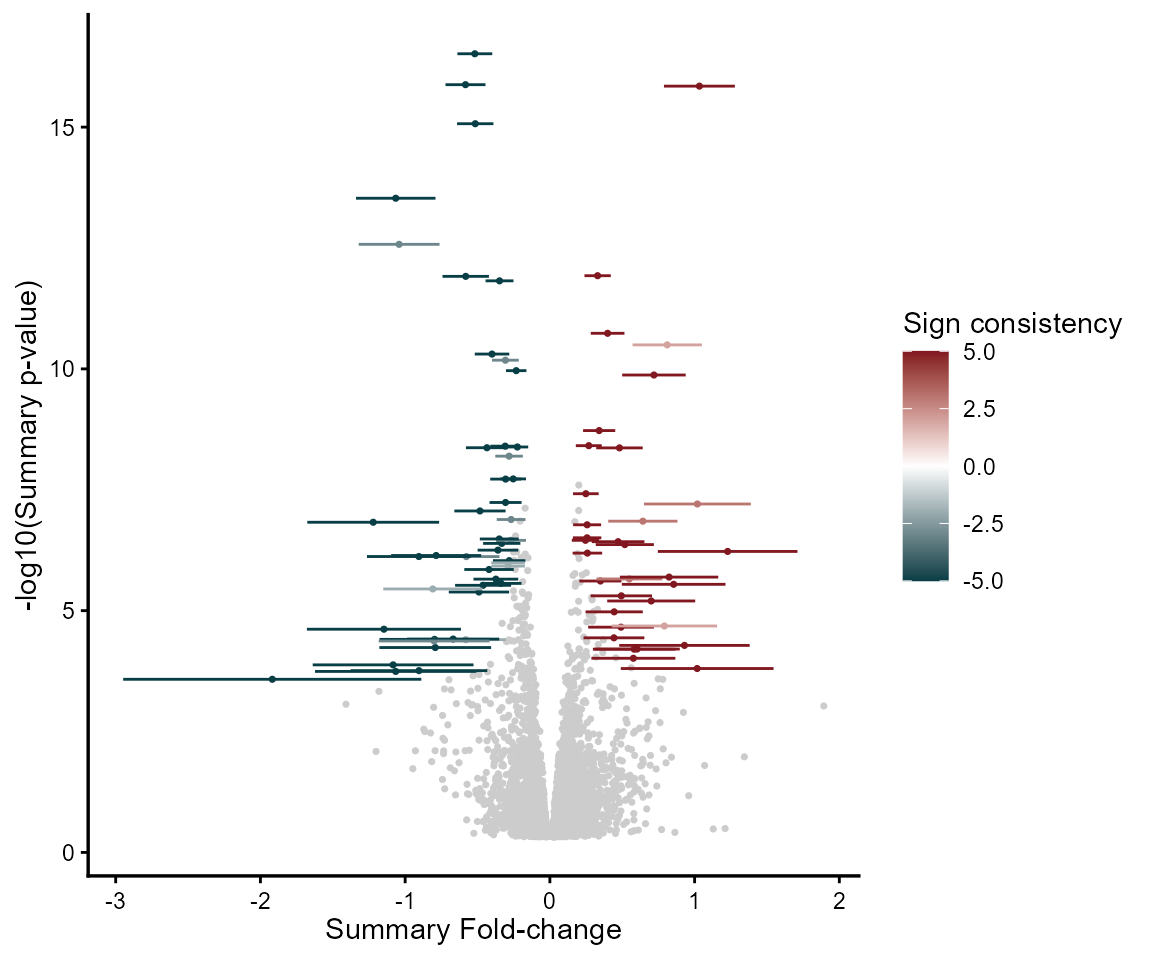

REM with labels and pseudogene filtering

When label_top_n is used, features are now ranked by the topconfects rank metric, which balances effect size and confidence.

mv_rem_labeled <- rem_mv(
  diffexp       = diffexplist,
  pcriteria     = "pvalue",
  foldchangecol = "Log2FC",
  genenamecol   = "Symbol",
  llcol         = "CI.L",
  rlcol         = "CI.R",
  metathr       = 0.01,
  label_top_n   = 10,
  label_size    = 3.5,
  plot_title    = "REM Meta-Analysis (Top 10)",
  show_legend   = TRUE,
  jobname       = "REM_labeled",
  outputfolder  = tempdir(),
  draw          = "HTML"
)

##   index  Symbol   Log2FC_1     CI.L_1     CI.R_1       vi_1   Log2FC_2
## 1  4795   MXRA5  0.8150851  0.3109324  1.3192377 0.06616251  1.3001104
## 2  2166  COL6A6 -1.7480348 -2.5780749 -0.9179947 0.17934364 -0.8388366
## 3  2053   CIDEA         NA         NA         NA         NA         NA
## 4  7115 SULT1A4  0.9689025  0.5103475  1.4274575 0.05473571  0.7513323
## 5   130   ACACB -0.8431142 -1.4708480 -0.2153804 0.10257437 -1.1119841
## 6  6528 SLC27A2 -0.6782948 -0.9931027 -0.3634869 0.02579759 -1.8916655
##       CI.L_2     CI.R_2       vi_2   Log2FC_3     CI.L_3     CI.R_3        vi_3
## 1  0.6603306  1.9398901 0.10654886  1.1895480  0.8401301  1.5389659 0.031781777
## 2 -1.3578456 -0.3198277 0.07011930 -1.0300519 -1.4730328 -0.5870710 0.051080819
## 3         NA         NA         NA -1.0111528 -1.3226326 -0.6996729 0.025255027
## 4  0.4707021  1.0319624 0.02050012         NA         NA         NA          NA
## 5 -1.7417389 -0.4822293 0.10323592 -0.5305046 -0.6957455 -0.3652637 0.007107599
## 6 -2.6822584 -1.1010726 0.16270229 -1.2126830 -1.6702908 -0.7550753 0.054509799
##     Log2FC_4    CI.L_4     CI.R_4      vi_4   Log2FC_5     CI.L_5     CI.R_5
## 1  0.2188594 -1.052230  1.4899492 0.4205720  0.8051543  0.1367255  1.4735830
## 2 -1.3755263 -2.162453 -0.5885999 0.1611967 -0.7213490 -1.5714484  0.1287505
## 3 -1.7991026 -2.918939 -0.6792665 0.3264351 -0.8738120 -1.6373061 -0.1103179
## 4         NA        NA         NA        NA         NA         NA         NA
## 5 -0.7991042 -1.457868 -0.1403403 0.1129659 -0.5155929 -0.8606782 -0.1705076
## 6 -1.3554403 -2.288444 -0.4224370 0.2265970 -1.4905464 -2.5565023 -0.4245905
##         vi_5 signcon ntimes randomSummary randomCi.lb randomCi.ub      randomP
## 1 0.11630493       5      5     1.0333001   0.7882044   1.2783958 1.420312e-16
## 2 0.18811668      -5      5    -1.0649749  -1.3396138  -0.7903361 2.956522e-14
## 3 0.15173972      -3      3    -1.0417876  -1.3210774  -0.7624977 2.653168e-13
## 4         NA       2      2     0.8106154   0.5712566   1.0499741 3.187477e-11
## 5 0.03099851      -5      5    -0.5830624  -0.7212245  -0.4449003 1.324963e-16
## 6 0.29577833      -5      5    -1.2207058  -1.6760435  -0.7653680 1.484852e-07
##      het_QE    het_QEp   het_QM      het_QMp error         se rank
## 1  4.179945 0.38220032 68.27752 1.420312e-16 FALSE 0.12504883    1
## 2  4.580708 0.33308457 57.76318 2.956522e-14 FALSE 0.14012185    2
## 3  1.980047 0.37156797 53.44957 2.653168e-13 FALSE 0.14249482    3
## 4  0.629179 0.42765661 44.05825 3.187477e-11 FALSE 0.12212181    4
## 5  4.317851 0.36469506 68.41455 1.324963e-16 FALSE 0.07049086    5
## 6 11.099093 0.02547263 27.60901 1.484852e-07 FALSE 0.23231516    6

mv_rem_labeled@MetaVolcano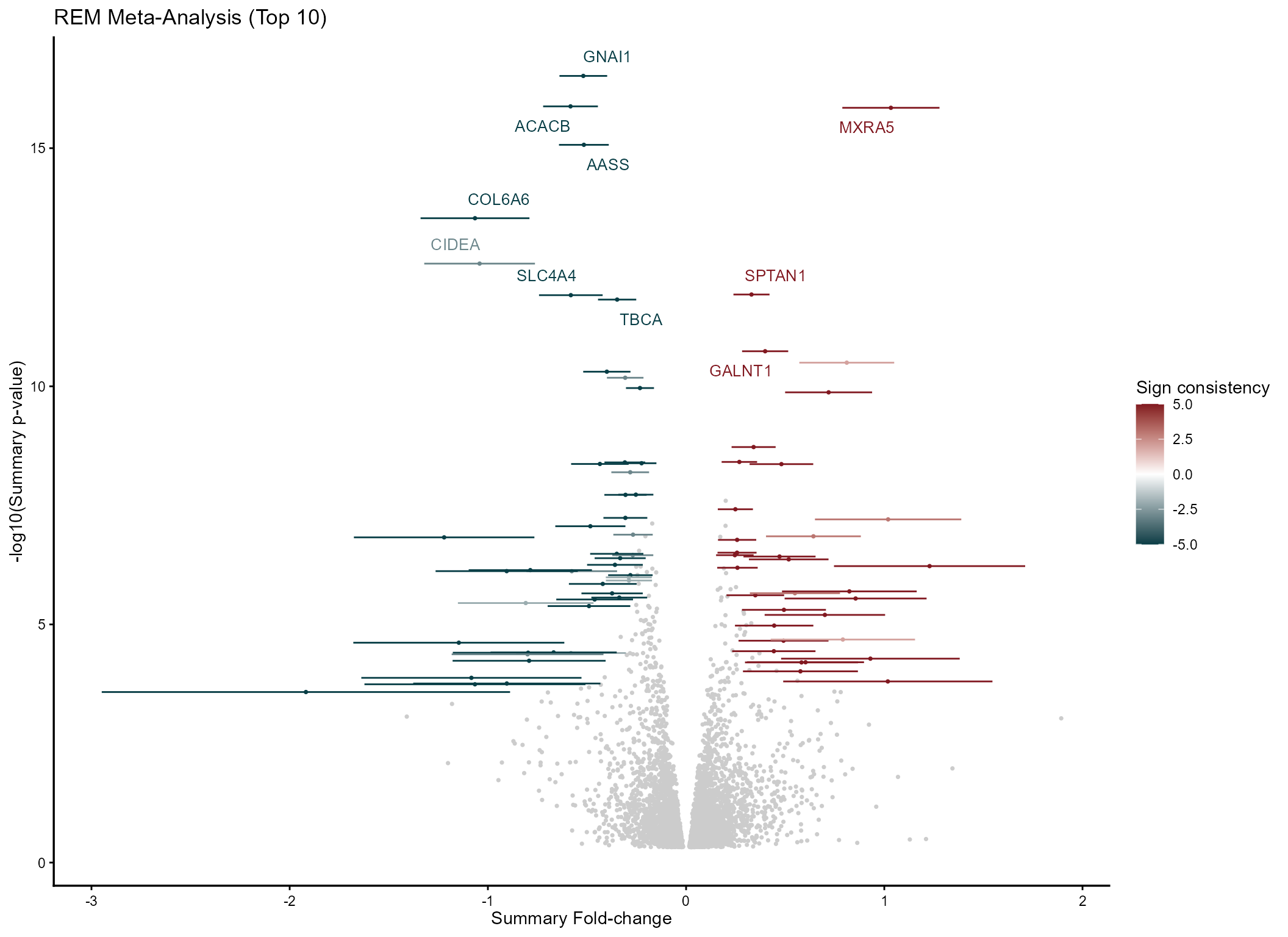

Custom colors

The colors parameter accepts a named vector for the sign consistency gradient:

mv_rem_custom <- rem_mv(
  diffexp       = diffexplist,
  pcriteria     = "pvalue",
  foldchangecol = "Log2FC",
  genenamecol   = "Symbol",
  llcol         = "CI.L",
  rlcol         = "CI.R",
  metathr       = 0.01,
  colors        = c(low = "purple", mid = "white", high = "orange", 
                    na = "gray80"),
  label_top_n   = 5,
  plot_title    = "REM with custom colors",
  jobname       = "REM_custom",
  outputfolder  = tempdir(),
  draw          = "HTML"
)

##   index  Symbol   Log2FC_1     CI.L_1     CI.R_1       vi_1   Log2FC_2
## 1  4795   MXRA5  0.8150851  0.3109324  1.3192377 0.06616251  1.3001104
## 2  2166  COL6A6 -1.7480348 -2.5780749 -0.9179947 0.17934364 -0.8388366
## 3  2053   CIDEA         NA         NA         NA         NA         NA
## 4  7115 SULT1A4  0.9689025  0.5103475  1.4274575 0.05473571  0.7513323
## 5   130   ACACB -0.8431142 -1.4708480 -0.2153804 0.10257437 -1.1119841
## 6  6528 SLC27A2 -0.6782948 -0.9931027 -0.3634869 0.02579759 -1.8916655
##       CI.L_2     CI.R_2       vi_2   Log2FC_3     CI.L_3     CI.R_3        vi_3
## 1  0.6603306  1.9398901 0.10654886  1.1895480  0.8401301  1.5389659 0.031781777
## 2 -1.3578456 -0.3198277 0.07011930 -1.0300519 -1.4730328 -0.5870710 0.051080819
## 3         NA         NA         NA -1.0111528 -1.3226326 -0.6996729 0.025255027
## 4  0.4707021  1.0319624 0.02050012         NA         NA         NA          NA
## 5 -1.7417389 -0.4822293 0.10323592 -0.5305046 -0.6957455 -0.3652637 0.007107599
## 6 -2.6822584 -1.1010726 0.16270229 -1.2126830 -1.6702908 -0.7550753 0.054509799
##     Log2FC_4    CI.L_4     CI.R_4      vi_4   Log2FC_5     CI.L_5     CI.R_5
## 1  0.2188594 -1.052230  1.4899492 0.4205720  0.8051543  0.1367255  1.4735830
## 2 -1.3755263 -2.162453 -0.5885999 0.1611967 -0.7213490 -1.5714484  0.1287505
## 3 -1.7991026 -2.918939 -0.6792665 0.3264351 -0.8738120 -1.6373061 -0.1103179
## 4         NA        NA         NA        NA         NA         NA         NA
## 5 -0.7991042 -1.457868 -0.1403403 0.1129659 -0.5155929 -0.8606782 -0.1705076
## 6 -1.3554403 -2.288444 -0.4224370 0.2265970 -1.4905464 -2.5565023 -0.4245905
##         vi_5 signcon ntimes randomSummary randomCi.lb randomCi.ub      randomP
## 1 0.11630493       5      5     1.0333001   0.7882044   1.2783958 1.420312e-16
## 2 0.18811668      -5      5    -1.0649749  -1.3396138  -0.7903361 2.956522e-14
## 3 0.15173972      -3      3    -1.0417876  -1.3210774  -0.7624977 2.653168e-13
## 4         NA       2      2     0.8106154   0.5712566   1.0499741 3.187477e-11
## 5 0.03099851      -5      5    -0.5830624  -0.7212245  -0.4449003 1.324963e-16
## 6 0.29577833      -5      5    -1.2207058  -1.6760435  -0.7653680 1.484852e-07
##      het_QE    het_QEp   het_QM      het_QMp error         se rank
## 1  4.179945 0.38220032 68.27752 1.420312e-16 FALSE 0.12504883    1
## 2  4.580708 0.33308457 57.76318 2.956522e-14 FALSE 0.14012185    2
## 3  1.980047 0.37156797 53.44957 2.653168e-13 FALSE 0.14249482    3
## 4  0.629179 0.42765661 44.05825 3.187477e-11 FALSE 0.12212181    4
## 5  4.317851 0.36469506 68.41455 1.324963e-16 FALSE 0.07049086    5
## 6 11.099093 0.02547263 27.60901 1.484852e-07 FALSE 0.23231516    6

mv_rem_custom@MetaVolcano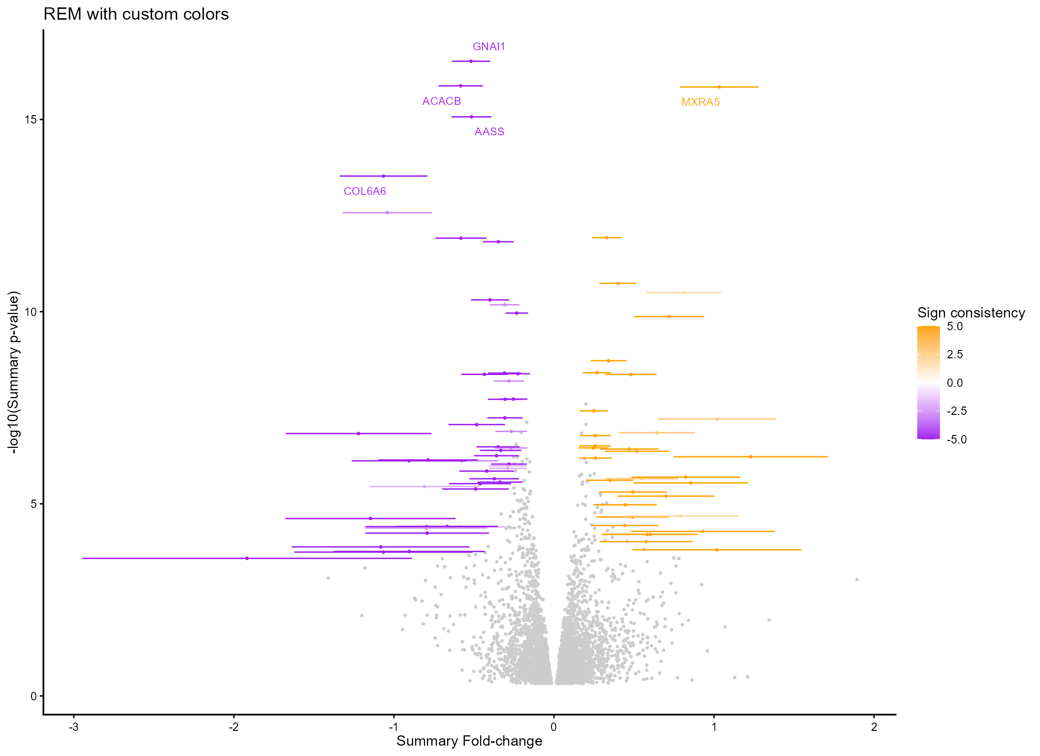

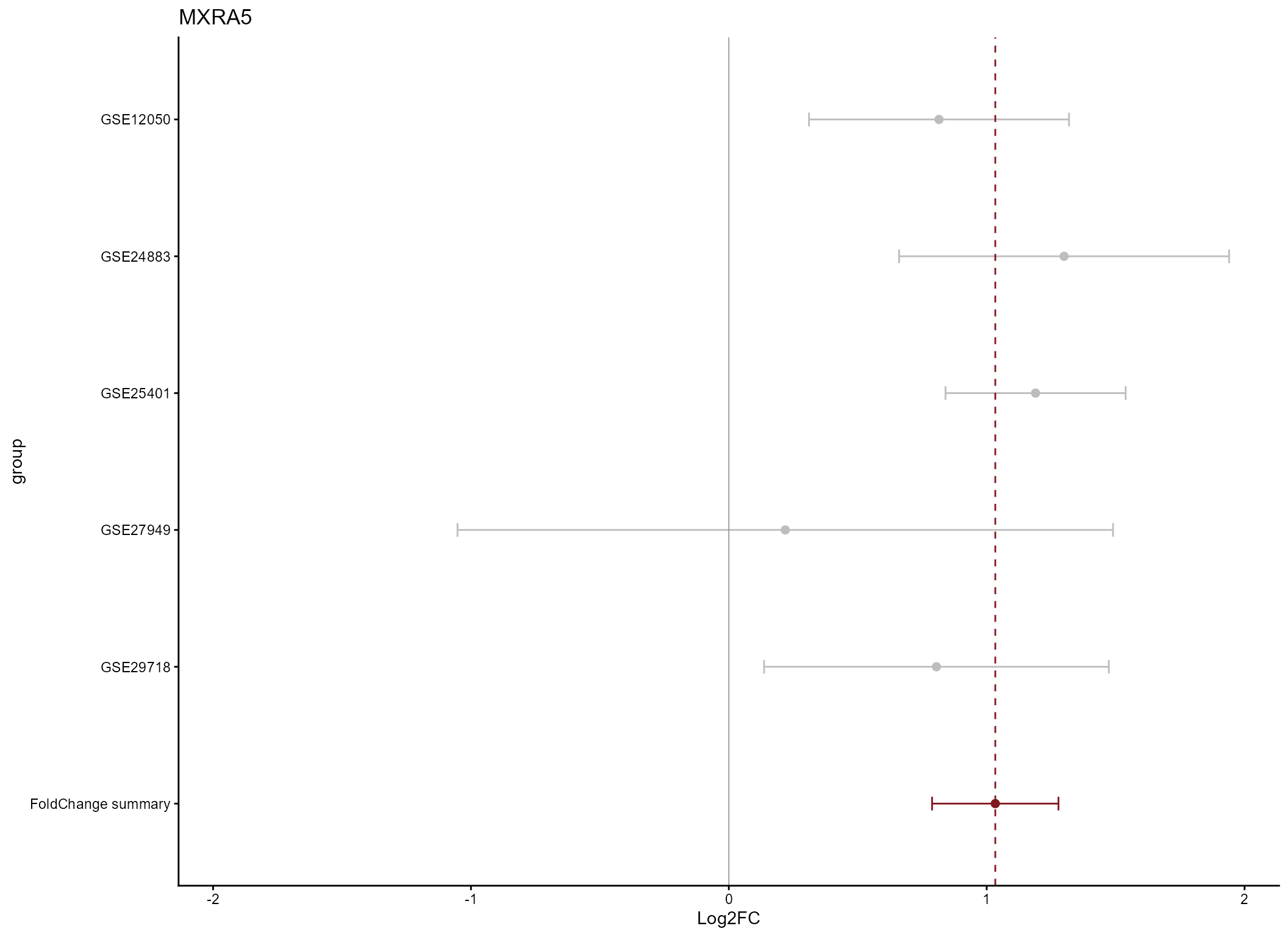
2. Forest Plots

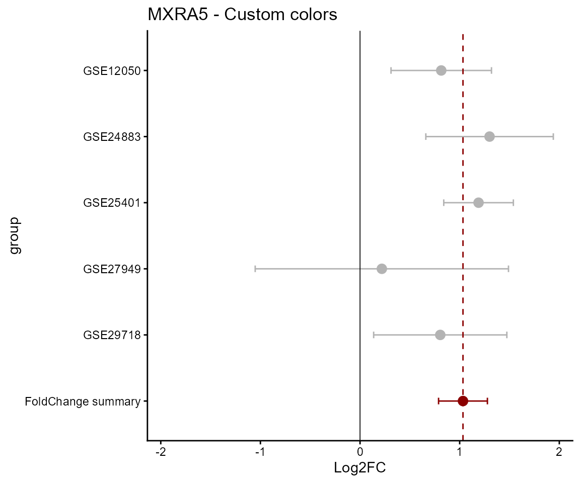
Forest plots now accept custom colors via a named vector:

# Top 3 features by rank
top3 <- mv_rem@metaresult %>%
  filter(!is.na(randomP)) %>%
  arrange(rank) %>%
  head(3) %>%
  pull(Symbol)

cat("Top 3 features:", paste(top3, collapse = ", "), "\n")

## Top 3 features: MXRA5, COL6A6, CIDEA

# Forest plot with default updated colors
draw_forest(
  remres        = mv_rem,
  gene          = top3[1],
  genecol       = "Symbol",
  foldchangecol = "Log2FC",
  llcol         = "CI.L",
  rlcol         = "CI.R",
  jobname       = "Forest_example",
  outputfolder  = tempdir(),
  draw          = "HTML"
)

Custom forest plot colors:

draw_forest(
  remres        = mv_rem,
  gene          = top3[1],
  genecol       = "Symbol",
  foldchangecol = "Log2FC",
  llcol         = "CI.L",
  rlcol         = "CI.R",
  colors        = c(positive = "darkred", negative = "steelblue",
                    neutral = "gray70", reference = "black"),
  point_size    = 3,
  plot_title    = paste(top3[1], "- Custom colors"),
  jobname       = "Forest_custom",
  outputfolder  = tempdir(),
  draw          = "HTML"
)

3. Vote-Counting

Fixed axis and improved labels

The vote-counting plot now uses scale_x_continuous for correct symmetric axis display. Labels are selected using abs(idx) — the package’s own combined metric of frequency and direction consistency (idx = ndeg × ddeg).

mv_vote <- votecount_mv(
  diffexp       = diffexplist,
  pcriteria     = "pvalue",
  foldchangecol = "Log2FC",
  genenamecol   = "Symbol",
  geneidcol     = NULL,
  pvalue        = 0.05,
  foldchange    = 0,
  metathr       = 0.01,
  label_top_n   = 10,
  label_size    = 3.5,
  plot_title    = "Vote-Counting (Top 10 by |idx|)",
  jobname       = "Vote_example",
  outputfolder  = tempdir(),
  draw          = "HTML"
)

mv_vote@MetaVolcano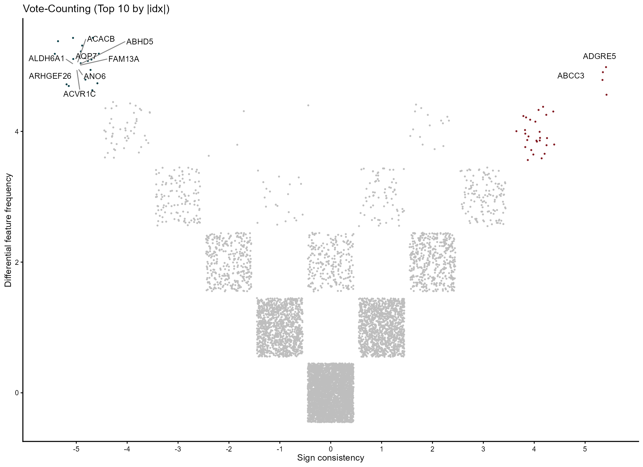

Label selection criteria

Previous behavior ranked labels by ndeg only (number of studies where DE). This could label features with inconsistent direction across studies.

The updated behavior uses abs(idx) and filters out unperturbed features:

Protein	ndeg	ddeg	idx	Previous rank	Updated rank
A	5	5	25	1st (tied)	1st
B	5	-5	-25	1st (tied)	2nd
C	5	1	5	1st (tied)	3rd

DEG barplot with custom colors

draw_featurebar() now accepts a colors parameter:

mv_vote@featurefreq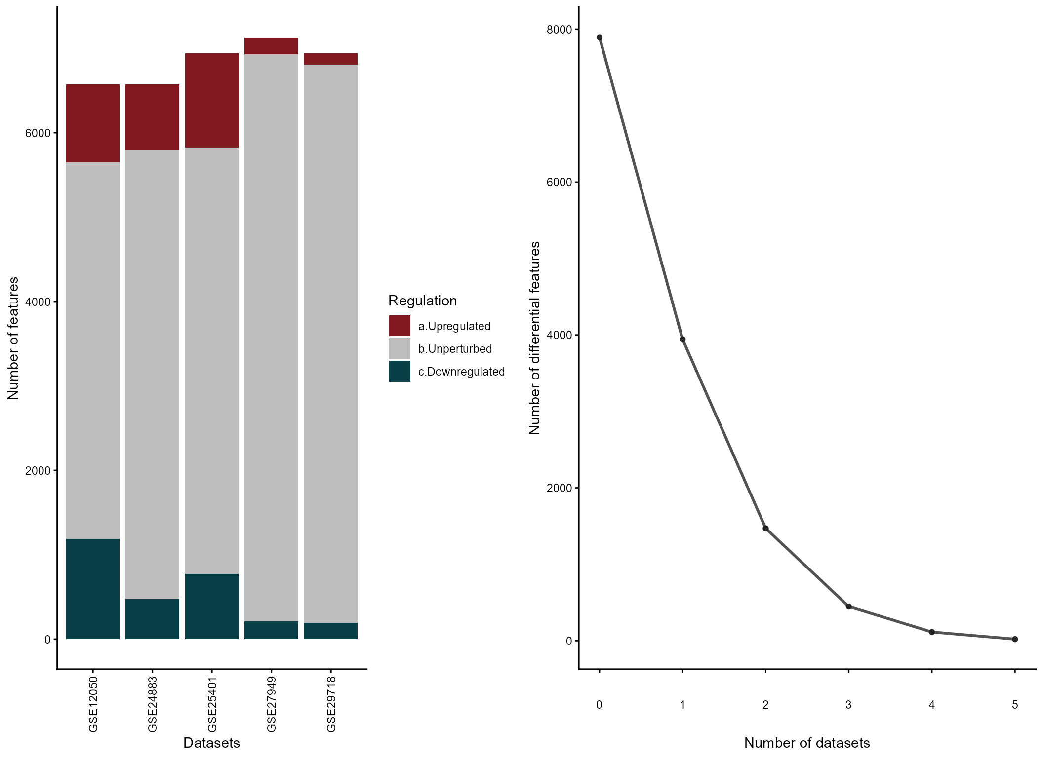

4. Combining (Fisher’s Method)

Fisher’s combining approach also supports the updated color palette:

mv_fisher <- combining_mv(
  diffexp       = diffexplist,
  pcriteria     = "pvalue",
  foldchangecol = "Log2FC",
  genenamecol   = "Symbol",
  metafc        = "Mean",
  metathr       = 0.01,
  colors        = c("#083e46", "gray90", "#811820"),
  point_size    = 1.2,
  show_legend   = TRUE,
  plot_title    = "Fisher's Combined Test",
  jobname       = "Fisher_example",
  outputfolder  = tempdir(),
  draw          = "HTML"
)

mv_fisher@MetaVolcano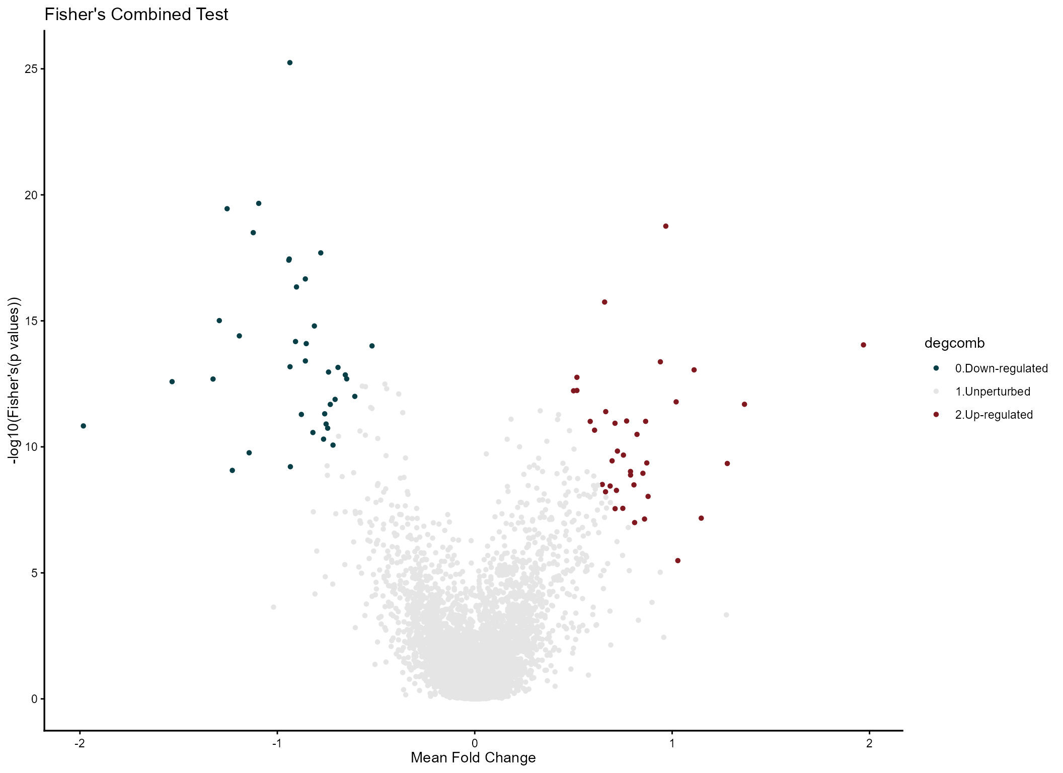

5. Functional Enrichment — `enrichment_mv()`

The new enrichment_mv() function wraps fGSEA and integrates directly with the REM MetaVolcano results. Gene sets can be provided manually or downloaded automatically from MSigDB.

Automatic MSigDB download

# GO Biological Process (default: category = "C5")
enrich <- enrichment_mv(mv_rem, subcategory = "GO:BP")
enrich$plot
head(enrich$result)

Three ranking strategies

# 1. Fold-change — prioritizes effect size
enrich_fc <- enrichment_mv(mv_rem, ranking = "fc")

# 2. Signed significance — prioritizes statistical confidence
enrich_sp <- enrichment_mv(mv_rem, ranking = "signed_p")

# 3. Weighted FC — balances both
enrich_wfc <- enrichment_mv(mv_rem, ranking = "weighted_fc")

Ranking	Formula	Best for
`fc`	randomSummary	Pathways with large effects
`signed_p`	-log10(p) × sign(FC)	Pathways with consistent significance
`weighted_fc`	FC × -log10(p)	Balanced detection

Selecting pathway databases

# KEGG pathways
enrich_kegg <- enrichment_mv(
  mv_rem,
  category    = "C2",
  subcategory = "CP:KEGG",
  ranking     = "weighted_fc"
)

# Hallmark features sets
enrich_hall <- enrichment_mv(
  mv_rem,
  category = "H"
)

# GO Molecular Function only
enrich_mf <- enrichment_mv(
  mv_rem,
  subcategory = "GO:MF"
)

Full customization

enrich <- enrichment_mv(
  mv_rem,
  category            = "C5",
  subcategory         = "GO:BP",
  ranking             = "weighted_fc",
  plot_padj           = 0.05,
  plot_top_n          = 20,
  clean_pathway_names = TRUE,
  colors              = c(down = "navy", up = "darkred"),
  plot_title          = "GO:BP Enrichment (weighted FC ranking)"
)

enrich$plot

Using custom features sets

my_pathways <- list(
  "INFLAMMATION"  = c("IL6", "TNF", "IL1B", "CXCL8", "CCL2"),
  "ANGIOGENESIS"  = c("VEGFA", "FLT1", "KDR", "ANGPT1"),
  "ECM_REMODEL"   = c("MMP2", "MMP9", "MMP12", "COL1A1")
)

enrich_custom <- enrichment_mv(
  mv_rem,
  pathways            = my_pathways,
  clean_pathway_names = FALSE
)

Izabela Mamede, Bárbara Marinho, Cesar Prada, Helder Nakaya

2026-07-13

Overview

Setup

1. Random Effects Model (REM)

Basic REM

REM with labels and pseudogene filtering

Custom colors

2. Forest Plots

3. Vote-Counting

Fixed axis and improved labels

Label selection criteria

DEG barplot with custom colors

4. Combining (Fisher’s Method)

5. Functional Enrichment — `enrichment_mv()`

Automatic MSigDB download

Three ranking strategies

Selecting pathway databases

Full customization

Using custom features sets

MetaVolcanoR: Updated Features and Enrichment Analysis

Izabela Mamede, Bárbara Marinho, Cesar Prada, Helder Nakaya

2026-07-13

Overview

Setup

1. Random Effects Model (REM)

Basic REM

REM with labels and pseudogene filtering

Custom colors

2. Forest Plots

3. Vote-Counting

Fixed axis and improved labels

Label selection criteria

DEG barplot with custom colors

4. Combining (Fisher’s Method)

5. Functional Enrichment — enrichment_mv()

Automatic MSigDB download

Three ranking strategies

Selecting pathway databases

Full customization

Using custom features sets

5. Functional Enrichment — `enrichment_mv()`