MetaVolcanoR: Differential expression meta-analysis tool

Introduction: Why Meta-Analysis?

Imagine you’re studying a disease and find 5 different studies on Gene Expression Omnibus, each identifying ~500 differentially expressed genes (DEGs). But only 50 genes overlap! Which genes are truly important?

MetaVolcanoR solves this by: - Combining evidence across studies - Identifying consistently perturbed genes - Visualizing meta-analysis results intuitively

Comparing the expression of genes under a given condition against a reference biological state is usually applied to identify sets of differentially expressed genes (DEG). These DEG point out the genomic regions functionally relevant under the biological condition of interest.

Athough individual genome-wide expression studies have small signal/noise ratio, today’s genomic data availability usually allows to combine differential gene expression results from dozens of independent studies to overcome this limitation.

Databases such as GEO (https://www.ncbi.nlm.nih.gov/geo/), SRA (https://www.ncbi.nlm.nih.gov/sra), ArrayExpress, (https://www.ebi.ac.uk/arrayexpress/), and ENA (https://www.ebi.ac.uk/ena) offer systematic access to vast amounts of transcriptome data. There exists more than one gene expression study for many biological conditions. This redundancy could be exploit by meta-analysis approaches to reveal genes that are consistently present and differentially expressed under given conditions.

MetaVolcanoR was designed to identify the genes whose expression is consistently perturbed across several DE tables.

Usage

Overview

The MetaVolcanoR R package combines differential gene expression results. It implements three strategies to summarize gene expression activities from different studies. i) Random Effects Model (REM) approach. ii) a vote-counting approach, and iii) a p-value combining-approach. MetaVolcano exploits the Volcano plot reasoning to visualize these meta-analysis of gene expression results.

Installation

Load library

library(MetaVolcanoR)

Preparing Your Data

MetaVolcanoR requires differential expression results with:

Gene identifiers (gene names or IDs)
Log2 fold changes
P-values
Confidence intervals OR variance (for REM method only)

If you have confidence intervals (CI)

If your DE results include confidence interval columns (example: CI.L and CI.R), you're ready to go! The package will automatically calculate variance:

# Your data has CI.L and CI.R columns
meta_rem <- rem_mv(
  diffexp = your_data_list,
  llcol = "CI.L",      # Left limit of CI
  rlcol = "CI.R",      # Right limit of CI
  cvar = TRUE          # Calculate variance from CI (default)
)

If you have standard error (SE)

Most tools (DESeq2, limma, edgeR) output standard error, not confidence intervals. Convert SE to 95% CI:

# From DESeq2 results
deseq_results <- results(dds) #or after shrinkage
deseq_results$CI.L <- deseq_results$log2FoldChange - 1.96 * deseq_results$lfcSE
deseq_results$CI.R <- deseq_results$log2FoldChange + 1.96 * deseq_results$lfcSE

# From limma results (if you have SE column)
limma_results$CI.L <- limma_results$logFC - 1.96 * limma_results$SE
limma_results$CI.R <- limma_results$logFC + 1.96 * limma_results$SE

If you have variance directly

If you have variance (or can calculate it from SE: variance = SE^2), use the vcol parameter:

# Calculate variance from standard error
your_data$variance <- your_data$SE^2

# Use variance directly
meta_rem <- rem_mv(
  diffexp = your_data_list,
  vcol = "variance",   # Column name with variance
  cvar = FALSE         # Don\'t calculate from CI
)

Estimating variance from test statistics

If your differential expression results do not include confidence interval columns, variance can be approximated from the fold-change and test statistic (e.g. z-score or t-statistic), using the relationship stat ≈ log2FC / SE, which gives var = (log2FC / stat)^2.

If your data is already organized as a named list of data frames, you can add the variance column as follows:

# If your tables are already in a list called diffexp_list:
diffexp_list <- lapply(diffexp_list, function(df) {
  df %>%
    mutate(var = ifelse(stat == 0 | is.na(stat), 
                        NA_real_, 
                        (log2FC / stat)^2))
})

Note the ifelse guard — transcripts where stat = 0 would produce infinite variance and cause rem_mv to fail, so these are set to NA and will be handled gracefully by the model (flagged as error = TRUE).

Then pass vcol = "var" and cvar = FALSE to rem_mv:

meta_mv <- rem_mv(
  diffexp = diffexp_list,
  pcriteria = "pvalue",
  foldchangecol = "log2FC",
  genenamecol = "Symbol",
  geneidcol = "Symbol",
  llcol = NULL,
  rlcol = NULL,
  vcol = "var",
  cvar = FALSE,
  ...
)

Preparing Swish/fishpond transcript-level results

If your differential expression analysis was performed at the transcript level using swish() from the fishpond package, MetaVolcanoR can integrate your results using an approximate estimate of variance derived from Swish’s test statistic. This lets you go straight from the differential transcript expression (DET) results table to a MetaVolcanoR-ready format, without needing to carry the SummarizedExperiment object or its inferential replicates forward.

Checking your DET table

Before preparing your data, inspect the columns available in your results table:

colnames(det)

swish() adds the following statistical result columns to rowData(): stat, log2FC, pvalue, locfdr, qvalue. If you extracted your DET table with something like det <- as.data.frame(mcols(se)), these columns carry over directly. Identifier columns (e.g. tx_id, tx_name) depend on how you imported your quantification data — if you used tximeta::tximeta(), these are typically added automatically based on the salmon index and usually contain Ensembl transcript IDs (e.g. ENST00000456328.2) rather than human-readable isoform names (e.g. HES4-202).

prepare_swish() auto-detects the identifier column by looking for tx_name, tx_id, transcript_id, or transcript_name (in that order) among your column names — no need to pass tx_col if one of these is present. If your identifier column has a different name, or if you plan to combine several studies with rem_mv(), pass tx_col explicitly and make sure the identifiers are consistent across all studies (same ID type, same versioning). Any ID harmonization should be done upstream, on your DET table, prior to this step.

Preparing swish results for MetaVolcanoR

Once your DET table has a consistent identifier column, use prepare_swish() to generate the table required by MetaVolcanoR:

# Auto-detects the identifier column (tx_name, tx_id, etc.)
det_table <- prepare_swish(det = det_1)

# Or specify explicitly if needed
det_table <- prepare_swish(det = det_1, tx_col = "tx_name")

If your identifiers are plain Ensembl transcript IDs, the Symbol column will simply contain values like ENST00000456328.2. The meta-analysis will still run without any issue — this only affects how gene/transcript labels look on the volcano plot:

det_table <- prepare_swish(det = det_1, tx_col = "tx_id")

Complete workflow with prepare_swish()

library(fishpond)
library(SummarizedExperiment)
library(MetaVolcanoR)

# Extract DET tables from your swish results
det_1 <- as.data.frame(mcols(se_swish_1))
det_2 <- as.data.frame(mcols(se_swish_2))

# Prepare each study
study_1 <- prepare_swish(det = det_1, tx_col = "tx_name")
study_2 <- prepare_swish(det = det_2, tx_col = "tx_name")

# Combine into named list — names are required
my_studies <- list(
  study1 = study_1,
  study2 = study_2
)

# Run REM meta-analysis
meta_results <- rem_mv(
  diffexp       = my_studies,
  pcriteria     = "pvalue",
  foldchangecol = "Log2FC",
  genenamecol   = "Symbol",
  llcol         = "CI.L",
  rlcol         = "CI.R",
  cvar          = TRUE,
  metathr       = 0.01,
  draw          = "HTML"
)

meta_results@MetaVolcano

Preparing reuslts from common DE tools

MetaVolcanoR provides convenient helper functions to prepare results from common DE tools:

# For DESeq2 results 
deg_table <- prepare_deseq2(res)

# For limma results
deg_table <- prepare_limma(limma_toptable)

# For edgeR results
deg_table <- prepare_edger(edger_toptags$table)

# For Swish/fishpond results (transcript-level)
det_table <- prepare_swish(det)

Complete workflow with helper functions:

library(DESeq2)
library(MetaVolcanoR)

# Run your DESeq2 analysis
dds <- DESeqDataSetFromMatrix(count_matrix, sample_info, design = ~ condition)
dds <- DESeq(dds)

# Get results for multiple comparisons
res_treatment1 <- results(dds, contrast = c("condition", "Treatment1", "Control"))
res_treatment2 <- results(dds, contrast = c("condition", "Treatment2", "Control"))
res_treatment3 <- results(dds, contrast = c("condition", "Treatment3", "Control"))

# Prepare all studies using helper function
study1 <- prepare_deseq2(res_treatment1)
study2 <- prepare_deseq2(res_treatment2)
study3 <- prepare_deseq2(res_treatment3)

# Combine into named list
my_studies <- list(
  "Treatment1_vs_Control" = study1,
  "Treatment2_vs_Control" = study2,
  "Treatment3_vs_Control" = study3
)

# Run meta-analysis
meta_results <- rem_mv(
  diffexp = my_studies,
  metathr = 0.01,
  outputfolder = tempdir(),
  draw = "HTML"
)

# View results
meta_results@MetaVolcano
head(meta_results@metaresult)

Testing the helper functions:

You can test if your data is correctly formatted:

# Load example data
data(diffexplist)

# Check the required columns
head(diffexplist[[1]])

##     Symbol      Log2FC      pvalue       CI.L        CI.R
## 1     A1BG -0.70126879 0.000140100 -1.0087857 -0.39375189
## 2 A1BG-AS1 -0.25106351 0.008694757 -0.4304790 -0.07164803
## 3     A1CF  0.03332573 0.615989488 -0.1036882  0.17033968
## 4      A2M  0.83504214 0.018550388  0.1568214  1.51326289
## 5    A2ML1  0.03942552 0.843222358 -0.3728473  0.45169836
## 6   A4GALT -0.20815882 0.282488068 -0.6025247  0.18620708

# Your prepared data should have these columns:
# - Symbol (or gene identifier)
# - Log2FC (fold change)
# - pvalue (p-value)
# - CI.L (lower confidence interval, for REM only)
# - CI.R (upper confidence interval, for REM only)

# Test with one study
str(diffexplist[[1]])

## 'data.frame':    6573 obs. of  5 variables:
##  $ Symbol: chr  "A1BG" "A1BG-AS1" "A1CF" "A2M" ...
##  $ Log2FC: num  -0.7013 -0.2511 0.0333 0.835 0.0394 ...
##  $ pvalue: num  0.00014 0.00869 0.61599 0.01855 0.84322 ...
##  $ CI.L  : num  -1.009 -0.43 -0.104 0.157 -0.373 ...
##  $ CI.R  : num  -0.3938 -0.0716 0.1703 1.5133 0.4517 ...
##  - attr(*, ".internal.selfref")=<externalptr>

Note: The prepare_* functions automatically: - Remove rows with NA values - Calculate 95% confidence intervals from standard errors - Format column names to match MetaVolcanoR requirements - Filter out infinite values

Implemented meta-analysis approaches

Random Effect Model MetaVolcano

The REM MetaVolcano summarizes the gene fold change of several studies taking into account the variance. The REM estimates a summary p-value which stands for the probability of the summary fold-change is not different than zero. Users can set the metathr parameter to highlight the top percentage of the most consistently perturbed genes. This perturbation ranking is defined following the topconfects approach.

meta_degs_rem <- rem_mv(diffexp=diffexplist,
            pcriteria="pvalue",
            foldchangecol='Log2FC', 
            genenamecol='Symbol',
            geneidcol=NULL,
            collaps=FALSE,
            llcol='CI.L',
            rlcol='CI.R',
            vcol=NULL, 
            cvar=TRUE,
            metathr=0.01,
            jobname="MetaVolcano",
            outputfolder=".", 
            draw='HTML',
            ncores=1)

##   index  Symbol   Log2FC_1     CI.L_1     CI.R_1       vi_1   Log2FC_2
## 1  4795   MXRA5  0.8150851  0.3109324  1.3192377 0.06616251  1.3001104
## 2  2166  COL6A6 -1.7480348 -2.5780749 -0.9179947 0.17934364 -0.8388366
## 3  2053   CIDEA         NA         NA         NA         NA         NA
## 4  7115 SULT1A4  0.9689025  0.5103475  1.4274575 0.05473571  0.7513323
## 5   130   ACACB -0.8431142 -1.4708480 -0.2153804 0.10257437 -1.1119841
## 6  6528 SLC27A2 -0.6782948 -0.9931027 -0.3634869 0.02579759 -1.8916655
##       CI.L_2     CI.R_2       vi_2   Log2FC_3     CI.L_3     CI.R_3        vi_3
## 1  0.6603306  1.9398901 0.10654886  1.1895480  0.8401301  1.5389659 0.031781777
## 2 -1.3578456 -0.3198277 0.07011930 -1.0300519 -1.4730328 -0.5870710 0.051080819
## 3         NA         NA         NA -1.0111528 -1.3226326 -0.6996729 0.025255027
## 4  0.4707021  1.0319624 0.02050012         NA         NA         NA          NA
## 5 -1.7417389 -0.4822293 0.10323592 -0.5305046 -0.6957455 -0.3652637 0.007107599
## 6 -2.6822584 -1.1010726 0.16270229 -1.2126830 -1.6702908 -0.7550753 0.054509799
##     Log2FC_4    CI.L_4     CI.R_4      vi_4   Log2FC_5     CI.L_5     CI.R_5
## 1  0.2188594 -1.052230  1.4899492 0.4205720  0.8051543  0.1367255  1.4735830
## 2 -1.3755263 -2.162453 -0.5885999 0.1611967 -0.7213490 -1.5714484  0.1287505
## 3 -1.7991026 -2.918939 -0.6792665 0.3264351 -0.8738120 -1.6373061 -0.1103179
## 4         NA        NA         NA        NA         NA         NA         NA
## 5 -0.7991042 -1.457868 -0.1403403 0.1129659 -0.5155929 -0.8606782 -0.1705076
## 6 -1.3554403 -2.288444 -0.4224370 0.2265970 -1.4905464 -2.5565023 -0.4245905
##         vi_5 signcon ntimes randomSummary randomCi.lb randomCi.ub      randomP
## 1 0.11630493       5      5     1.0333001   0.7882044   1.2783958 1.420312e-16
## 2 0.18811668      -5      5    -1.0649749  -1.3396138  -0.7903361 2.956522e-14
## 3 0.15173972      -3      3    -1.0417876  -1.3210774  -0.7624977 2.653168e-13
## 4         NA       2      2     0.8106154   0.5712566   1.0499741 3.187477e-11
## 5 0.03099851      -5      5    -0.5830624  -0.7212245  -0.4449003 1.324963e-16
## 6 0.29577833      -5      5    -1.2207058  -1.6760435  -0.7653680 1.484852e-07
##      het_QE    het_QEp   het_QM      het_QMp error         se rank
## 1  4.179945 0.38220032 68.27752 1.420312e-16 FALSE 0.12504883    1
## 2  4.580708 0.33308457 57.76318 2.956522e-14 FALSE 0.14012185    2
## 3  1.980047 0.37156797 53.44957 2.653168e-13 FALSE 0.14249482    3
## 4  0.629179 0.42765661 44.05825 3.187477e-11 FALSE 0.12212181    4
## 5  4.317851 0.36469506 68.41455 1.324963e-16 FALSE 0.07049086    5
## 6 11.099093 0.02547263 27.60901 1.484852e-07 FALSE 0.23231516    6

head(meta_degs_rem@metaresult, 3)

##   Symbol signcon randomSummary randomCi.lb randomCi.ub      randomP   het_QE
## 1  MXRA5       5      1.033300   0.7882044   1.2783958 1.420312e-16 4.179945
## 2 COL6A6      -5     -1.064975  -1.3396138  -0.7903361 2.956522e-14 4.580708
## 3  CIDEA      -3     -1.041788  -1.3210774  -0.7624977 2.653168e-13 1.980047
##     het_QEp   het_QM      het_QMp error rank
## 1 0.3822003 68.27752 1.420312e-16 FALSE    1
## 2 0.3330846 57.76318 2.956522e-14 FALSE    2
## 3 0.3715680 53.44957 2.653168e-13 FALSE    3

meta_degs_rem@MetaVolcano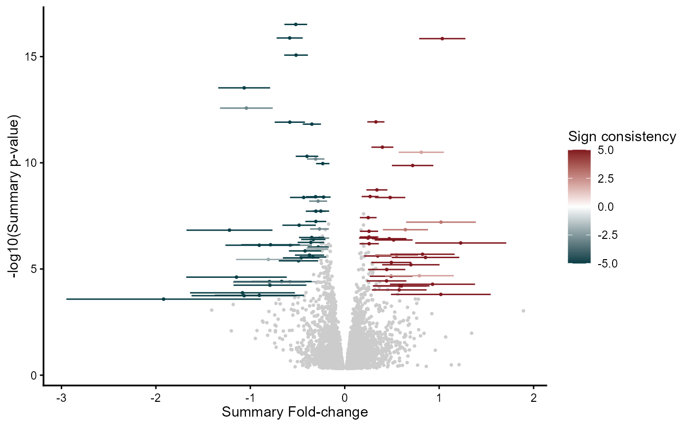

draw_forest(remres=meta_degs_rem,
        gene="MMP9",
        genecol="Symbol", 
        foldchangecol="Log2FC",
        llcol="CI.L", 
        rlcol="CI.R",
        jobname="MetaVolcano",
        outputfolder=".",
        draw="HTML")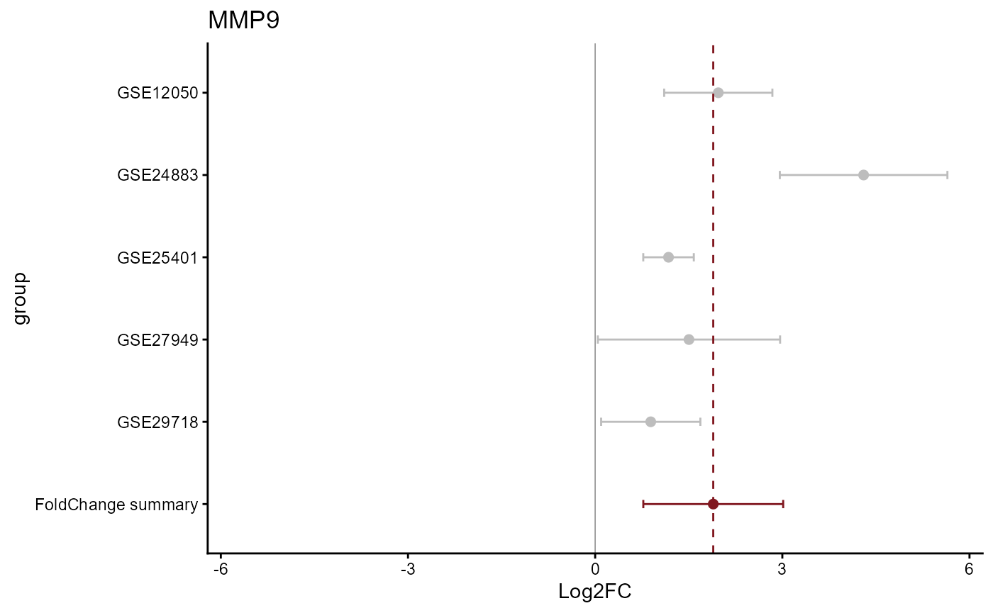

draw_forest(remres=meta_degs_rem,
        gene="COL6A6",
        genecol="Symbol", 
        foldchangecol="Log2FC",
        llcol="CI.L", 
        rlcol="CI.R",
        jobname="MetaVolcano",
        outputfolder=".",
        draw="HTML")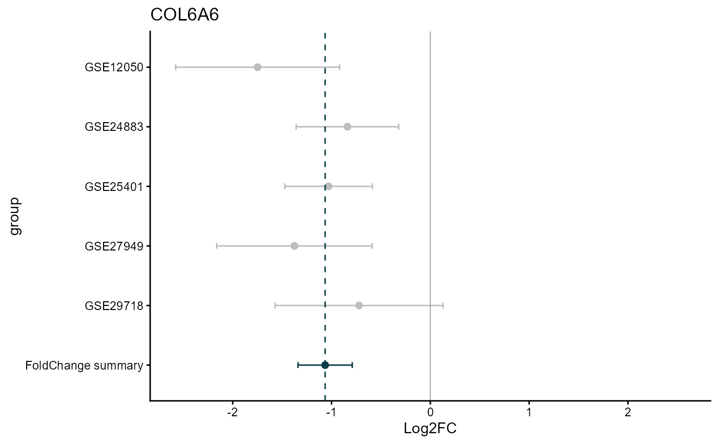

The REM MetaVolcano also allows users to explore the forest plot of a given gene based on the REM results.

Vote-counting approach

The vote-counting MetaVolcano identifies differential expressed genes (DEG) for each study based on the user-defined p-value and fold change thresholds. It displays the number of differentially expressed and unperturbed genes per study. In addition, it plots the inverse cumulative distribution of the consistently DEG, so the user can identify the number of genes whose expression is perturbed in at least 1 or n studies.

meta_degs_vote <- votecount_mv(diffexp=diffexplist,
                   pcriteria='pvalue',
                   foldchangecol='Log2FC',
                   genenamecol='Symbol',
                   geneidcol=NULL,
                   pvalue=0.05,
                   foldchange=0, 
                   metathr=0.01,
                   collaps=FALSE,
                   jobname="MetaVolcano", 
                   outputfolder=".",
                   draw='HTML')

head(meta_degs_vote@metaresult, 3)

##   Symbol deg_1 deg_2 deg_3 deg_4 deg_5 ndeg ddeg idx        degvcount
## 1  ABCC3     1     1     1     1     1    5    5  25   2.Up-regulated
## 2  ABHD5    -1    -1    -1    -1    -1    5   -5 -25 0.Down-regulated
## 3  ACACB    -1    -1    -1    -1    -1    5   -5 -25 0.Down-regulated

meta_degs_vote@featurefreq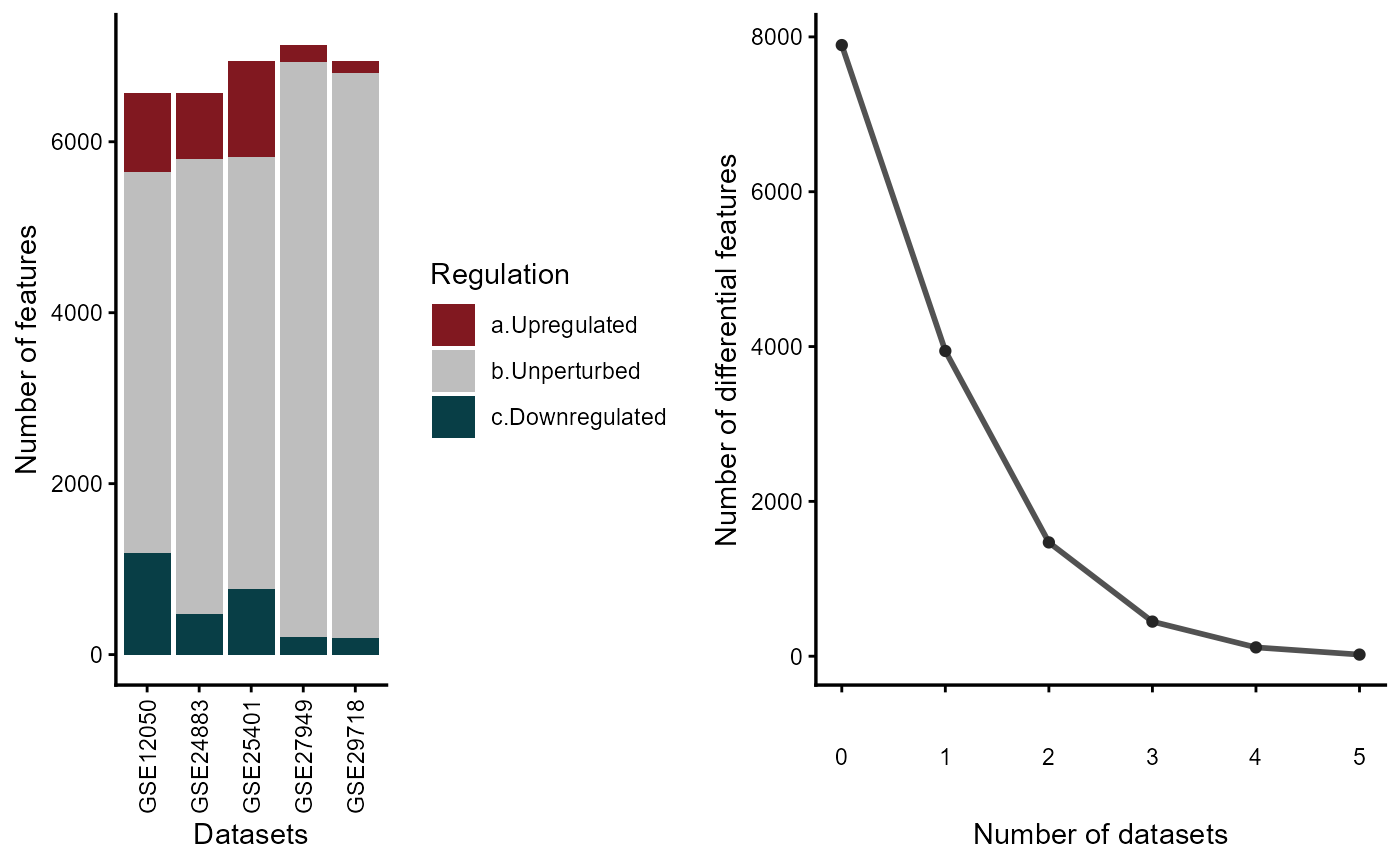

The vote-counting MetaVolcano visualizes genes based on the number of studies where genes were identified as differentially expressed and the gene fold change sign consistency. It means that a gene that was differentially expressed in five studies, from which three of them it was downregulated, will get a sign consistency score of 2 + (-3) = -1. Based on user preference, MetaVolcano can highlight the top metathr percentage of consistently perturbed genes.

meta_degs_vote@MetaVolcano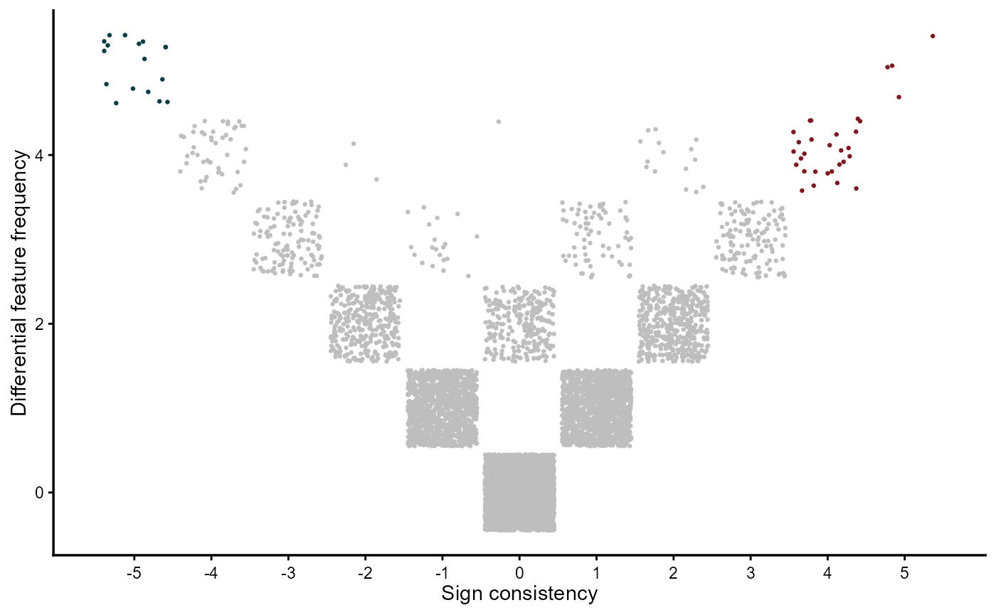

Combining-approach

The combinig MetaVolcano summarizes the fold change of a gene in different studies by the mean or median depending on the user preference. In addition, the combinig MetaVolcano summarizes the gene differential expression p-values using the Fisher method. The combining MetaVolcano can highlight the top metathr percentage of consistently perturbed genes.

meta_degs_comb <- combining_mv(diffexp=diffexplist,
                   pcriteria='pvalue', 
                   foldchangecol='Log2FC',
                   genenamecol='Symbol',
                   geneidcol=NULL,
                   metafc='Mean',
                   metathr=0.01, 
                   collaps=TRUE,
                   jobname="MetaVolcano",
                   outputfolder=".",
                   draw='HTML')

head(meta_degs_comb@metaresult, 3)

##   Symbol        metap     metafc       idx
## 1   MMP9 9.002947e-15  1.9693517  27.66076
## 2 ACVR1C 3.548802e-20 -1.2544105 -24.39818
## 3    ANG 5.674270e-26 -0.9364936 -23.64280

meta_degs_comb@MetaVolcano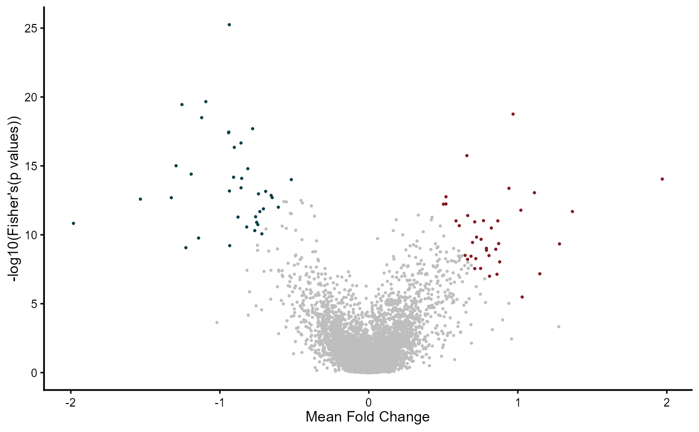

Customizing Your Plots

MetaVolcanoR provides extensive customization options to create publication-ready figures and highlight specific genes of interest.

Basic Customization Options

All main functions (rem_mv, votecount_mv, combining_mv) support these parameters:

colors: Custom color schemes
point_size: Size of data points
label_genes: Vector of specific genes to label
label_top_n: Automatically label top N genes
label_size: Size of gene labels
plot_title: Custom plot title
show_legend: Show or hide legend

Example 1: Custom Colors and Gene Labels

# REM with custom colors and specific genes labeled
meta_custom <- rem_mv(
  diffexp = diffexplist,
  metathr = 0.01,
  outputfolder = tempdir(),
  draw = "HTML",
  # Customization parameters:
  colors = c(low = "navy", mid = "white", high = "darkred", na = "gray80"),
  point_size = 1.5,
  label_genes = c("MMP9", "COL6A6", "MXRA5", "CIDEA"),
  label_size = 4,
  plot_title = "REM Meta-Analysis - Custom Colors",
  show_legend = TRUE
)

meta_custom@MetaVolcano

Example 2: Highlighting Top Genes Automatically

# Vote-counting with automatic labeling of top 10 genes
meta_vote_labeled <- votecount_mv(
  diffexp = diffexplist,
  pvalue = 0.05,
  metathr = 0.01,
  outputfolder = tempdir(),
  draw = "HTML",
  # Automatically label top 10 most significant genes
  colors = c("steelblue", "gray90", "firebrick"),
  point_size = 1.2,
  label_top_n = 10,
  label_size = 3.5,
  plot_title = "Vote-Counting: Top 10 DEGs Labeled"
)

meta_vote_labeled@MetaVolcano

Example 3: Publication-Ready Figures

# Combining approach with publication styling
meta_publication <- combining_mv(
  diffexp = diffexplist,
  metafc = "Median",
  metathr = 0.01,
  collaps = TRUE,
  outputfolder = tempdir(),
  draw = "HTML",
  # Publication-ready styling
  colors = c("darkgreen", "white", "darkorange"),
  point_size = 1.0,
  label_genes = c("MMP9", "ANG", "ACVR1C"),
  label_size = 3,
  plot_title = NULL,  # No title for publication
  show_legend = FALSE
)

meta_publication@MetaVolcano

Example 4: Customizing Forest Plots

Forest plots also support extensive customization:

# Custom forest plot with specific colors and dimensions
draw_forest(
  remres = meta_degs_rem,
  gene = "MMP9",
  outputfolder = tempdir(),
  draw = "PDF",
  # Customization:
  colors = c(
    positive = "darkred",    # Color for positive fold changes
    negative = "steelblue",  # Color for negative fold changes
    neutral = "gray70",      # Color for individual studies
    reference = "black"      # Color for reference lines
  ),
  point_size = 3,
  plot_width = 7,          # Width in inches (for PDF)
  plot_height = 6,         # Height in inches
  plot_title = "MMP9 Expression Meta-Analysis"
)

Color Scheme Examples

Color Schemes for Different Contexts

# Professional/Conservative
colors_professional <- c(low = "blue", mid = "white", high = "red", na = "gray80")

# High Contrast (for presentations)
colors_presentation <- c(low = "purple", mid = "white", high = "orange", na = "lightgray")

# Color-blind friendly
colors_colorblind <- c(low = "#0072B2", mid = "white", high = "#D55E00", na = "gray80")

# Grayscale (for print)
colors_grayscale <- c(low = "black", mid = "gray90", high = "gray30", na = "gray70")

# Use any of these:
meta_rem <- rem_mv(
  diffexp = diffexplist,
  colors = colors_colorblind,  # Or any other scheme
  # ... other parameters
)

Vote-counting and Combining Colors

For vote-counting and combining approaches, provide a vector of 3 colors:

# Custom colors: [downregulated, neutral, upregulated]
custom_colors <- c("navyblue", "gray85", "darkred")

meta_vote <- votecount_mv(
  diffexp = diffexplist,
  colors = custom_colors,
  # ... other parameters
)

Combining Multiple Customizations

# Complete customization example
meta_final <- rem_mv(
  diffexp = diffexplist,
  metathr = 0.01,
  outputfolder = tempdir(),
  draw = "HTML",
  ncores = 4,
  # All customization options
  colors = c(low = "#0072B2", mid = "white", high = "#D55E00", na = "gray80"),
  point_size = 1.5,
  label_genes = c("MMP9", "COL6A6"),  # Label specific genes
  label_top_n = 5,                    # Also label top 5
  label_size = 3.5,
  plot_title = "Meta-Analysis: Disease vs Control",
  show_legend = TRUE
)

# Access the customized plot
meta_final@MetaVolcano

# View the forest plot for a specific gene
draw_forest(
  remres = meta_final,
  gene = "MMP9",
  outputfolder = tempdir(),
  draw = "PDF",
  colors = c(positive = "#D55E00", negative = "#0072B2", 
            neutral = "gray60", reference = "black"),
  point_size = 3,
  plot_width = 8,
  plot_height = 6
)

Tips for Publication-Quality Figures

Use color-blind friendly palettes (see examples above)
Set show_legend = FALSE for cleaner figures (add legend in figure caption)
Label only key genes instead of showing all labels
Use plot_title = NULL and add titles in your manuscript
Save as PDF (draw = "PDF") for vector graphics in publications
Adjust plot_width and plot_height to match journal requirements
Use consistent colors across all figures in your paper

Saving Plots Separately

If you want to save plots with specific dimensions without displaying them:

# Generate the meta-analysis
meta_result <- rem_mv(
  diffexp = diffexplist,
  draw = "HTML",  # or "PDF"
  outputfolder = "path/to/output",
  # ... other parameters
)

# The plot is automatically saved to the outputfolder
# For HTML: interactive plot you can explore in browser
# For PDF: publication-ready vector graphics

Feb 1, 2026