MetaVolcanoR: gene and transcript-level meta-analysis

📄 See also: Protein-level meta-analysis — CPTAC pan-cancer example

Introduction: Why Meta-Analysis?
- Overview
- Load library
Preparing Your Data
Implemented meta-analysis approaches
Additional example: differentially methylated probes
Customizing your plots

Introduction: Why Meta-Analysis?

Imagine you’re studying a disease and find 5 different studies on Gene Expression Omnibus, each identifying ~500 differentially expressed genes (DEGs). But only 50 genes overlap! Which genes are truly important?

MetaVolcanoR solves this by:

Combining evidence across studies
Identifying consistently perturbed genes
Visualizing meta-analysis results intuitively

Comparing the expression of genes under a given condition against a reference biological state is usually applied to identify sets of differentially expressed genes (DEG). These DEG point out the genomic regions functionally relevant under the biological condition of interest.

Although individual genome-wide expression studies have small signal/noise ratio, today’s genomic data availability usually allows combining differential gene expression results from dozens of independent studies to overcome this limitation.

Databases such as GEO, SRA, ArrayExpress, and ENA offer systematic access to vast amounts of transcriptome data. There exists more than one gene expression study for many biological conditions. This redundancy can be exploited by meta-analysis approaches to reveal genes that are consistently and differentially expressed under given conditions.

MetaVolcanoR was designed to identify the genes whose expression is consistently perturbed across several DE tables, and — as this vignette also shows — it applies just as well to other feature types (transcripts, methylation probes) that share the same identifier / log-fold-change / p-value / confidence-interval structure.

Overview

The MetaVolcanoR R package combines differential expression results across studies. It implements three strategies to summarize differential activity from different studies:

Random Effects Model (REM) — weights each study by the inverse of its variance and estimates a summary fold-change and summary p-value per feature.
A p-value combining approach — combines per-study p-values with Fisher’s method and summarizes the fold-change by mean or median.
A vote-counting approach — counts, per feature, how many studies call it differentially expressed and in which direction.

In all three, MetaVolcanoR exploits the volcano-plot reasoning to visualize the meta-analysis result. All plots below use the package’s default styling; a dedicated Customizing your plots section at the end covers colors, titles, and labeling in depth.

Load library

library(MetaVolcanoR)
library(dplyr)
library(ggplot2)

Preparing Your Data

MetaVolcanoR requires differential expression results with:

Feature identifiers (gene names, transcript IDs, probe IDs, …)
Log2 fold changes
P-values
Confidence intervals OR variance (for the REM method only)

MetaVolcanoR only ever needs those four fields — what changes is how you get there from whatever tool you already used. Find your scenario below and jump straight to it; each tab shows only the code relevant to that path, so you don’t need to read the others.

Already have a DEG table with a confidence interval (CI.L/CI.R) computed → CI ready
Already have a DEG table with standard error (SE), no CI → Standard error (SE)
Already have variance computed directly → Variance directly
Only have a test statistic (z or t), no CI/SE/variance → Test statistic (z or t)
Ran DESeq2 → DESeq2
Ran limma → limma
Ran edgeR → edgeR
Ran Swish/fishpond (transcript-level) → Swish/fishpond
Downloaded a table from NCBI GEO2R → GEO2R

What do you have?

CI ready

If your DE results already include confidence interval columns (e.g. CI.L and CI.R), you’re ready to go — the package will automatically calculate variance from them:

# Your data has CI.L and CI.R columns
meta_rem <- rem_mv(
  diffexp = your_data_list,
  llcol   = "CI.L",   # Left limit of CI
  rlcol   = "CI.R",   # Right limit of CI
  cvar    = TRUE      # Calculate variance from CI (default)
)

Standard error (SE)

Most tools (DESeq2, limma, edgeR) output standard error, not confidence intervals. Convert SE to a 95% CI:

# From DESeq2 results
deseq_results <- results(dds)  # or after shrinkage
deseq_results$CI.L <- deseq_results$log2FoldChange - 1.96 * deseq_results$lfcSE
deseq_results$CI.R <- deseq_results$log2FoldChange + 1.96 * deseq_results$lfcSE

# From limma results (if you have an SE column)
limma_results$CI.L <- limma_results$logFC - 1.96 * limma_results$SE
limma_results$CI.R <- limma_results$logFC + 1.96 * limma_results$SE

Variance directly

If you have variance (or can calculate it from SE: variance = SE^2), use the vcol parameter instead:

your_data$variance <- your_data$SE^2

meta_rem <- rem_mv(
  diffexp = your_data_list,
  vcol    = "variance",  # Column name with variance
  cvar    = FALSE        # Don't calculate from CI
)

Test statistic (z or t)

If your DE results have no confidence interval columns, variance can be approximated from the fold-change and the test statistic (e.g. z-score or moderated t-statistic), using stat ≈ log2FC / SE, which gives var = (log2FC / stat)^2:

diffexp_list <- lapply(diffexp_list, function(df) {
  df %>%
    mutate(var = ifelse(stat == 0 | is.na(stat),
                        NA_real_,
                        (log2FC / stat)^2))
})

The ifelse guard matters: transcripts where stat = 0 would otherwise produce infinite variance and cause rem_mv() to fail. Setting them to NA lets the model skip them gracefully (they come back flagged error = TRUE in the result, rather than aborting the whole run).

meta_mv <- rem_mv(
  diffexp       = diffexp_list,
  pcriteria     = "pvalue",
  foldchangecol = "log2FC",
  genenamecol   = "Symbol",
  geneidcol     = "Symbol",
  llcol         = NULL,
  rlcol         = NULL,
  vcol          = "var",
  cvar          = FALSE
)

DESeq2

prepare_deseq2() maps a DESeqResults object straight into MetaVolcanoR’s format.

library(DESeq2)
library(MetaVolcanoR)

dds <- DESeqDataSetFromMatrix(count_matrix, sample_info, design = ~ condition)
dds <- DESeq(dds)

res_treatment1 <- results(dds, contrast = c("condition", "Treatment1", "Control"))
res_treatment2 <- results(dds, contrast = c("condition", "Treatment2", "Control"))
res_treatment3 <- results(dds, contrast = c("condition", "Treatment3", "Control"))

study1 <- prepare_deseq2(res_treatment1)
study2 <- prepare_deseq2(res_treatment2)
study3 <- prepare_deseq2(res_treatment3)

my_studies <- list(
  "Treatment1_vs_Control" = study1,
  "Treatment2_vs_Control" = study2,
  "Treatment3_vs_Control" = study3
)

meta_results <- rem_mv(diffexp = my_studies, metathr = 0.01,
                        outputfolder = tempdir(), draw = "HTML")
meta_results@MetaVolcano
head(meta_results@metaresult)

limma

prepare_limma() maps a limma::topTable() output straight into MetaVolcanoR’s format.

library(limma)
library(MetaVolcanoR)

fit <- eBayes(lmFit(expr, design))
limma_toptable <- topTable(fit, coef = 2, number = Inf, confint = TRUE)

study1 <- prepare_limma(limma_toptable)

edgeR

prepare_edger() maps an edgeR topTags()$table straight into MetaVolcanoR’s format.

library(edgeR)
library(MetaVolcanoR)

et  <- exactTest(dge)
tt  <- topTags(et, n = Inf)

study1 <- prepare_edger(tt$table)

Swish/fishpond (transcript-level)

If your differential expression analysis was performed at the transcript level using swish() from the fishpond package, prepare_swish() maps your results table straight into MetaVolcanoR’s format, deriving an approximate variance from Swish’s test statistic — no need to carry the SummarizedExperiment object or its inferential replicates forward.

swish() adds stat, log2FC, pvalue, locfdr, qvalue to rowData(). If you extracted your table with det <- as.data.frame(mcols(se)), these columns carry over directly.

library(fishpond)
library(SummarizedExperiment)

det_1 <- as.data.frame(mcols(se_swish_1))
det_2 <- as.data.frame(mcols(se_swish_2))

# Auto-detects the identifier column (tx_name, tx_id, transcript_id, transcript_name)
study_1 <- prepare_swish(det = det_1)
study_2 <- prepare_swish(det = det_2, tx_col = "tx_name")  # or specify explicitly

my_studies <- list(study1 = study_1, study2 = study_2)

meta_results <- rem_mv(
  diffexp       = my_studies,
  pcriteria     = "pvalue",
  foldchangecol = "Log2FC",
  genenamecol   = "Symbol",
  llcol         = "CI.L",
  rlcol         = "CI.R",
  cvar          = TRUE,
  metathr       = 0.01,
  draw          = "HTML"
)

If your identifiers are plain Ensembl transcript IDs, the Symbol column will contain values like ENST00000456328.2. The meta-analysis still runs fine — this only affects how labels look on the plot.

GEO2R

GEO holds thousands of independent studies of comparable conditions, and NCBI’s GEO2R runs a limma differential-expression analysis on any suitable series directly in the browser, exporting a standardized table (Gene.symbol, logFC, P.Value, t, …). prepare_geo2r() maps that table to MetaVolcanoR’s format, deriving the 95% CI from the moderated t-statistic (SE = logFC / t), so a plain GEO2R export can feed the REM without any manual reformatting:

geo_tab <- read.delim("GSE12345.top.table.tsv", stringsAsFactors = FALSE)
study_1 <- prepare_geo2r(geo_tab)
head(study_1)

# Combine three independent GEO2R tables
diffexplist_geo <- lapply(list(GSE1 = tab1, GSE2 = tab2, GSE3 = tab3), prepare_geo2r)

meta_geo <- rem_mv(
  diffexp       = diffexplist_geo,
  pcriteria     = "pvalue",
  foldchangecol = "Log2FC",
  genenamecol   = "Symbol",
  llcol         = "CI.L",
  rlcol         = "CI.R",
  cvar          = TRUE,
  jobname       = "GEO2R",
  draw          = "PDF"
)

Note: the prepare_* functions automatically remove rows with NA values, calculate 95% confidence intervals where possible, format column names to MetaVolcanoR’s expected structure, and filter out infinite values. All of them converge on the same four columns (Symbol, Log2FC, pvalue, and CI.L/CI.R), so once your studies are prepared, the rest of the workflow below is identical no matter which tool they came from.

Checking your data is correctly formatted

data(diffexplist)
head(diffexplist[[1]])

##     Symbol      Log2FC      pvalue       CI.L        CI.R
## 1     A1BG -0.70126879 0.000140100 -1.0087857 -0.39375189
## 2 A1BG-AS1 -0.25106351 0.008694757 -0.4304790 -0.07164803
## 3     A1CF  0.03332573 0.615989488 -0.1036882  0.17033968
## 4      A2M  0.83504214 0.018550388  0.1568214  1.51326289
## 5    A2ML1  0.03942552 0.843222358 -0.3728473  0.45169836
## 6   A4GALT -0.20815882 0.282488068 -0.6025247  0.18620708

str(diffexplist[[1]])

## 'data.frame':    6573 obs. of  5 variables:
##  $ Symbol: chr  "A1BG" "A1BG-AS1" "A1CF" "A2M" ...
##  $ Log2FC: num  -0.7013 -0.2511 0.0333 0.835 0.0394 ...
##  $ pvalue: num  0.00014 0.00869 0.61599 0.01855 0.84322 ...
##  $ CI.L  : num  -1.009 -0.43 -0.104 0.157 -0.373 ...
##  $ CI.R  : num  -0.3938 -0.0716 0.1703 1.5133 0.4517 ...
##  - attr(*, ".internal.selfref")=<externalptr>

Your prepared data should have these columns: Symbol (or another feature identifier), Log2FC, pvalue, and — for the REM method — CI.L/CI.R.

cat("Number of datasets:", length(diffexplist), "\n")

## Number of datasets: 5

cat("Genes per dataset:",
    paste(sapply(diffexplist, nrow), collapse = ", "), "\n")

## Genes per dataset: 6573, 6573, 6944, 7131, 6944

Implemented meta-analysis approaches

1. Random Effects Model (REM)

The REM MetaVolcano summarizes the fold-change of a feature across several studies, taking the per-study variance into account, and estimates a summary p-value — the probability that the summary fold-change is not different from zero. The metathr parameter highlights the top percentage of most consistently perturbed features, ranked using the topconfects approach.

Since the current package version, the REM result also reports randomP.adjust: randomP corrected for multiple testing across all meta-analyzed features (Benjamini-Hochberg by default; configurable via the fdr_method argument — see ?rem_mv). Use randomP.adjust, not the nominal randomP, for feature selection and for functional enrichment (see below).

mv_rem <- rem_mv(
  diffexp       = diffexplist,
  pcriteria     = "pvalue",
  foldchangecol = "Log2FC",
  genenamecol   = "Symbol",
  llcol         = "CI.L",
  rlcol         = "CI.R",
  metathr       = 0.01,
  jobname       = "REM_example",
  outputfolder  = tempdir(),
  draw          = "HTML"
)

##   index  Symbol   Log2FC_1     CI.L_1     CI.R_1       vi_1   Log2FC_2
## 1  4795   MXRA5  0.8150851  0.3109324  1.3192377 0.06616251  1.3001104
## 2  2166  COL6A6 -1.7480348 -2.5780749 -0.9179947 0.17934364 -0.8388366
## 3  2053   CIDEA         NA         NA         NA         NA         NA
## 4  7115 SULT1A4  0.9689025  0.5103475  1.4274575 0.05473571  0.7513323
## 5   130   ACACB -0.8431142 -1.4708480 -0.2153804 0.10257437 -1.1119841
## 6  6528 SLC27A2 -0.6782948 -0.9931027 -0.3634869 0.02579759 -1.8916655
##       CI.L_2     CI.R_2       vi_2   Log2FC_3     CI.L_3     CI.R_3        vi_3
## 1  0.6603306  1.9398901 0.10654886  1.1895480  0.8401301  1.5389659 0.031781777
## 2 -1.3578456 -0.3198277 0.07011930 -1.0300519 -1.4730328 -0.5870710 0.051080819
## 3         NA         NA         NA -1.0111528 -1.3226326 -0.6996729 0.025255027
## 4  0.4707021  1.0319624 0.02050012         NA         NA         NA          NA
## 5 -1.7417389 -0.4822293 0.10323592 -0.5305046 -0.6957455 -0.3652637 0.007107599
## 6 -2.6822584 -1.1010726 0.16270229 -1.2126830 -1.6702908 -0.7550753 0.054509799
##     Log2FC_4    CI.L_4     CI.R_4      vi_4   Log2FC_5     CI.L_5     CI.R_5
## 1  0.2188594 -1.052230  1.4899492 0.4205720  0.8051543  0.1367255  1.4735830
## 2 -1.3755263 -2.162453 -0.5885999 0.1611967 -0.7213490 -1.5714484  0.1287505
## 3 -1.7991026 -2.918939 -0.6792665 0.3264351 -0.8738120 -1.6373061 -0.1103179
## 4         NA        NA         NA        NA         NA         NA         NA
## 5 -0.7991042 -1.457868 -0.1403403 0.1129659 -0.5155929 -0.8606782 -0.1705076
## 6 -1.3554403 -2.288444 -0.4224370 0.2265970 -1.4905464 -2.5565023 -0.4245905
##         vi_5 signcon ntimes randomSummary randomCi.lb randomCi.ub      randomP
## 1 0.11630493       5      5     1.0333001   0.7882044   1.2783958 1.420312e-16
## 2 0.18811668      -5      5    -1.0649749  -1.3396138  -0.7903361 2.956522e-14
## 3 0.15173972      -3      3    -1.0417876  -1.3210774  -0.7624977 2.653168e-13
## 4         NA       2      2     0.8106154   0.5712566   1.0499741 3.187477e-11
## 5 0.03099851      -5      5    -0.5830624  -0.7212245  -0.4449003 1.324963e-16
## 6 0.29577833      -5      5    -1.2207058  -1.6760435  -0.7653680 1.484852e-07
##      het_QE    het_QEp   het_QM      het_QMp error randomP.adjust         se
## 1  4.179945 0.38220032 68.27752 1.420312e-16 FALSE   3.737313e-13 0.12504883
## 2  4.580708 0.33308457 57.76318 2.956522e-14 FALSE   4.667756e-11 0.14012185
## 3  1.980047 0.37156797 53.44957 2.653168e-13 FALSE   3.490685e-10 0.14249482
## 4  0.629179 0.42765661 44.05825 3.187477e-11 FALSE   2.287450e-08 0.12212181
## 5  4.317851 0.36469506 68.41455 1.324963e-16 FALSE   3.737313e-13 0.07049086
## 6 11.099093 0.02547263 27.60901 1.484852e-07 FALSE   3.255949e-05 0.23231516
##   rank
## 1    1
## 2    2
## 3    3
## 4    4
## 5    5
## 6    6

head(mv_rem@metaresult, 3)

##   Symbol signcon randomSummary randomCi.lb randomCi.ub      randomP   het_QE
## 1  MXRA5       5      1.033300   0.7882044   1.2783958 1.420312e-16 4.179945
## 2 COL6A6      -5     -1.064975  -1.3396138  -0.7903361 2.956522e-14 4.580708
## 3  CIDEA      -3     -1.041788  -1.3210774  -0.7624977 2.653168e-13 1.980047
##     het_QEp   het_QM      het_QMp error randomP.adjust rank
## 1 0.3822003 68.27752 1.420312e-16 FALSE   3.737313e-13    1
## 2 0.3330846 57.76318 2.956522e-14 FALSE   4.667756e-11    2
## 3 0.3715680 53.44957 2.653168e-13 FALSE   3.490685e-10    3

mv_rem@MetaVolcano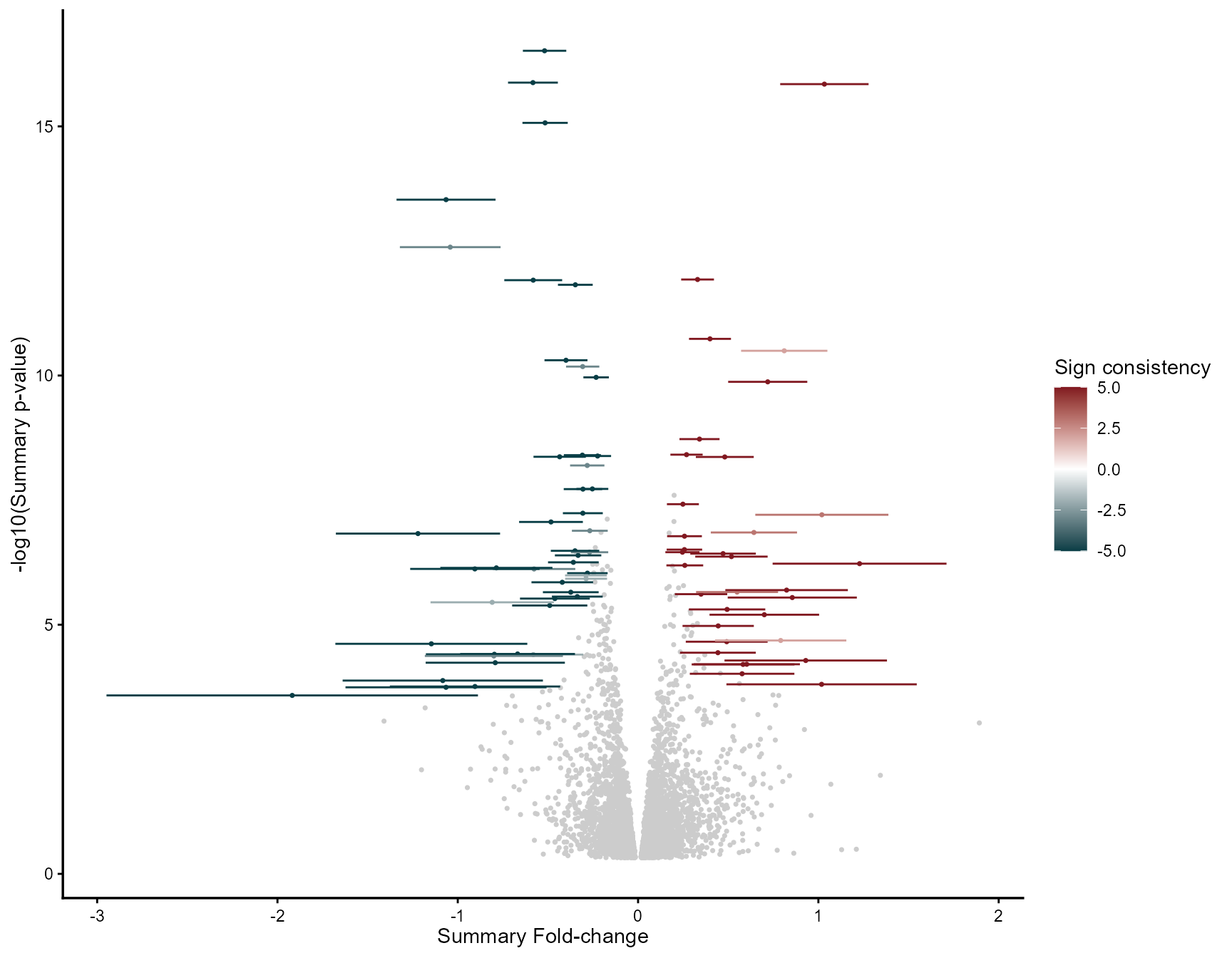

Labeling top features

When label_top_n is used, features are ranked by the topconfects rank metric, which balances effect size and confidence, rather than by fold-change or p-value alone:

mv_rem_labeled <- rem_mv(
  diffexp       = diffexplist,
  pcriteria     = "pvalue",
  foldchangecol = "Log2FC",
  genenamecol   = "Symbol",
  llcol         = "CI.L",
  rlcol         = "CI.R",
  metathr       = 0.01,
  label_top_n   = 10,
  label_size    = 3.5,
  jobname       = "REM_labeled",
  outputfolder  = tempdir(),
  draw          = "HTML"
)

##   index  Symbol   Log2FC_1     CI.L_1     CI.R_1       vi_1   Log2FC_2
## 1  4795   MXRA5  0.8150851  0.3109324  1.3192377 0.06616251  1.3001104
## 2  2166  COL6A6 -1.7480348 -2.5780749 -0.9179947 0.17934364 -0.8388366
## 3  2053   CIDEA         NA         NA         NA         NA         NA
## 4  7115 SULT1A4  0.9689025  0.5103475  1.4274575 0.05473571  0.7513323
## 5   130   ACACB -0.8431142 -1.4708480 -0.2153804 0.10257437 -1.1119841
## 6  6528 SLC27A2 -0.6782948 -0.9931027 -0.3634869 0.02579759 -1.8916655
##       CI.L_2     CI.R_2       vi_2   Log2FC_3     CI.L_3     CI.R_3        vi_3
## 1  0.6603306  1.9398901 0.10654886  1.1895480  0.8401301  1.5389659 0.031781777
## 2 -1.3578456 -0.3198277 0.07011930 -1.0300519 -1.4730328 -0.5870710 0.051080819
## 3         NA         NA         NA -1.0111528 -1.3226326 -0.6996729 0.025255027
## 4  0.4707021  1.0319624 0.02050012         NA         NA         NA          NA
## 5 -1.7417389 -0.4822293 0.10323592 -0.5305046 -0.6957455 -0.3652637 0.007107599
## 6 -2.6822584 -1.1010726 0.16270229 -1.2126830 -1.6702908 -0.7550753 0.054509799
##     Log2FC_4    CI.L_4     CI.R_4      vi_4   Log2FC_5     CI.L_5     CI.R_5
## 1  0.2188594 -1.052230  1.4899492 0.4205720  0.8051543  0.1367255  1.4735830
## 2 -1.3755263 -2.162453 -0.5885999 0.1611967 -0.7213490 -1.5714484  0.1287505
## 3 -1.7991026 -2.918939 -0.6792665 0.3264351 -0.8738120 -1.6373061 -0.1103179
## 4         NA        NA         NA        NA         NA         NA         NA
## 5 -0.7991042 -1.457868 -0.1403403 0.1129659 -0.5155929 -0.8606782 -0.1705076
## 6 -1.3554403 -2.288444 -0.4224370 0.2265970 -1.4905464 -2.5565023 -0.4245905
##         vi_5 signcon ntimes randomSummary randomCi.lb randomCi.ub      randomP
## 1 0.11630493       5      5     1.0333001   0.7882044   1.2783958 1.420312e-16
## 2 0.18811668      -5      5    -1.0649749  -1.3396138  -0.7903361 2.956522e-14
## 3 0.15173972      -3      3    -1.0417876  -1.3210774  -0.7624977 2.653168e-13
## 4         NA       2      2     0.8106154   0.5712566   1.0499741 3.187477e-11
## 5 0.03099851      -5      5    -0.5830624  -0.7212245  -0.4449003 1.324963e-16
## 6 0.29577833      -5      5    -1.2207058  -1.6760435  -0.7653680 1.484852e-07
##      het_QE    het_QEp   het_QM      het_QMp error randomP.adjust         se
## 1  4.179945 0.38220032 68.27752 1.420312e-16 FALSE   3.737313e-13 0.12504883
## 2  4.580708 0.33308457 57.76318 2.956522e-14 FALSE   4.667756e-11 0.14012185
## 3  1.980047 0.37156797 53.44957 2.653168e-13 FALSE   3.490685e-10 0.14249482
## 4  0.629179 0.42765661 44.05825 3.187477e-11 FALSE   2.287450e-08 0.12212181
## 5  4.317851 0.36469506 68.41455 1.324963e-16 FALSE   3.737313e-13 0.07049086
## 6 11.099093 0.02547263 27.60901 1.484852e-07 FALSE   3.255949e-05 0.23231516
##   rank
## 1    1
## 2    2
## 3    3
## 4    4
## 5    5
## 6    6

mv_rem_labeled@MetaVolcano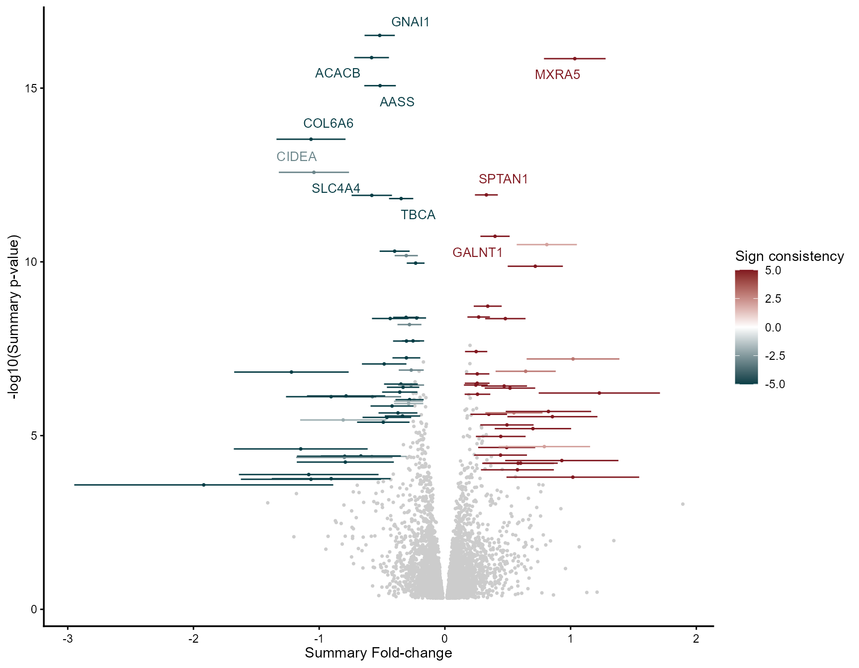

Forest plots

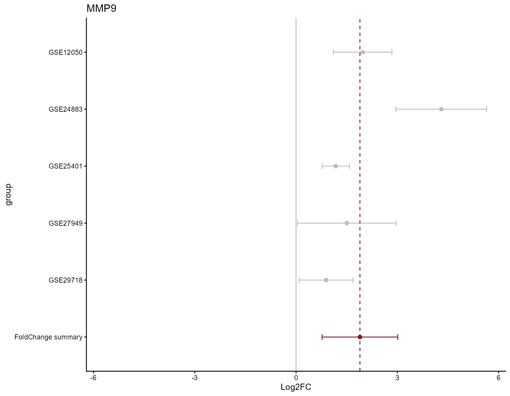
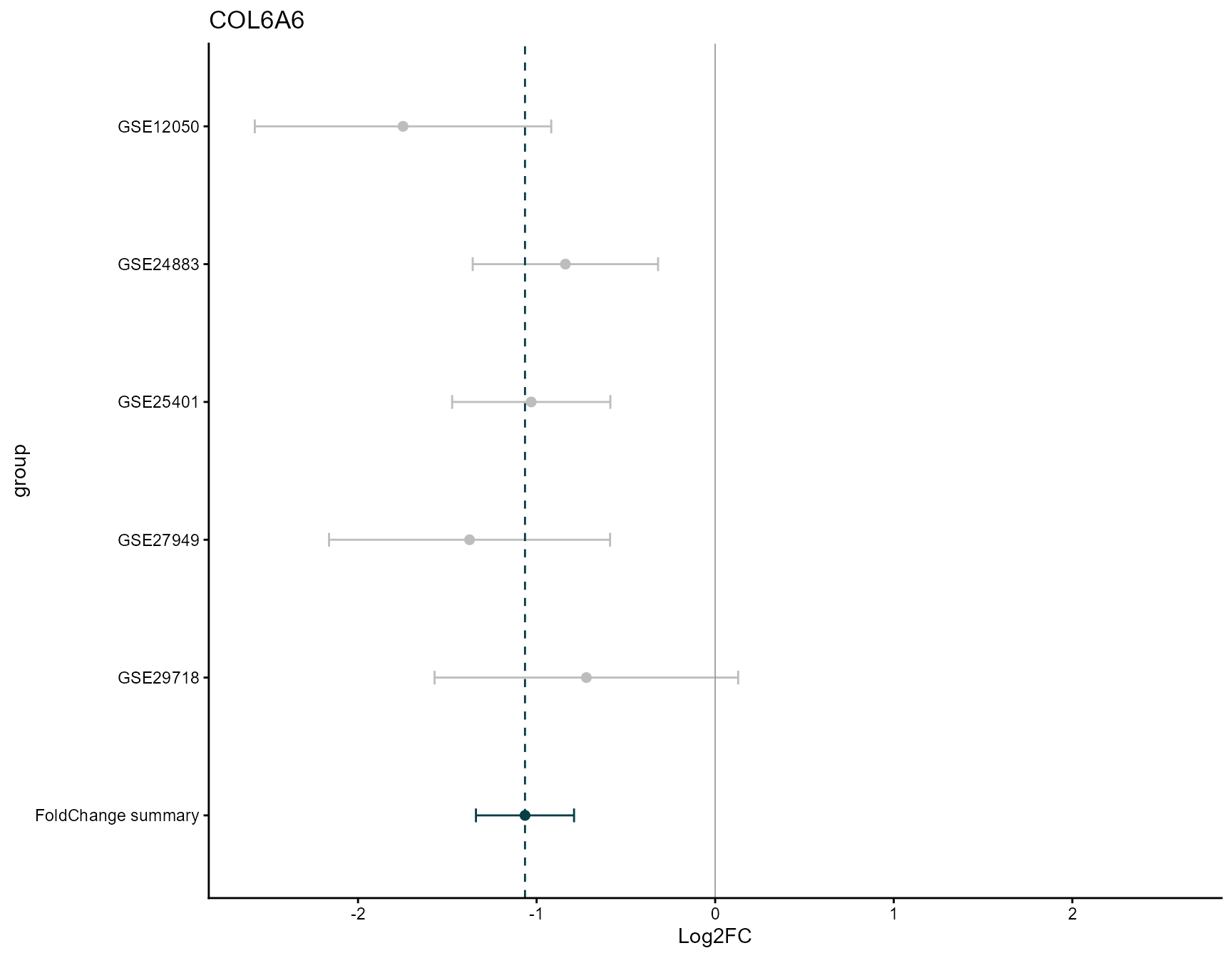
draw_forest() shows the per-study fold-change and confidence interval behind the REM summary for a single feature. Below, one consistently up-regulated feature (MMP9) and one consistently down-regulated feature (COL6A6):

draw_forest(
  remres        = mv_rem,
  gene          = "MMP9",
  genecol       = "Symbol",
  foldchangecol = "Log2FC",
  llcol         = "CI.L",
  rlcol         = "CI.R",
  jobname       = "MetaVolcano",
  outputfolder  = tempdir(),
  draw          = "HTML"
)

draw_forest(
  remres        = mv_rem,
  gene          = "COL6A6",
  genecol       = "Symbol",
  foldchangecol = "Log2FC",
  llcol         = "CI.L",
  rlcol         = "CI.R",
  jobname       = "MetaVolcano",
  outputfolder  = tempdir(),
  draw          = "HTML"
)

2. Vote-counting approach

The vote-counting MetaVolcano identifies differentially expressed features per study, based on user-defined p-value and fold-change thresholds, and displays how many studies call each feature differentially expressed and in which direction. A feature perturbed in five studies, three of them downregulated, gets a sign-consistency score of 2 + (-3) = -1.

Labels are selected using abs(idx) — the package’s own combined metric of frequency and direction consistency (idx = ndeg × ddeg) — rather than ndeg alone, which avoids labeling features with inconsistent direction across studies just because they were tested often:

Feature	ndeg	ddeg	idx	Rank by `ndeg` alone	Rank by `abs(idx)`
A	5	5	25	1st (tied)	1st
B	5	-5	-25	1st (tied)	2nd
C	5	1	5	1st (tied)	3rd

mv_vote <- votecount_mv(
  diffexp       = diffexplist,
  pcriteria     = "pvalue",
  foldchangecol = "Log2FC",
  genenamecol   = "Symbol",
  geneidcol     = NULL,
  pvalue        = 0.05,
  foldchange    = 0,
  metathr       = 0.01,
  label_top_n   = 10,
  label_size    = 3.5,
  jobname       = "Vote_example",
  outputfolder  = tempdir(),
  draw          = "HTML"
)

head(mv_vote@metaresult, 3)

##   Symbol deg_1 deg_2 deg_3 deg_4 deg_5 ndeg ddeg idx        degvcount
## 1  ABCC3     1     1     1     1     1    5    5  25   2.Up-regulated
## 2  ABHD5    -1    -1    -1    -1    -1    5   -5 -25 0.Down-regulated
## 3  ACACB    -1    -1    -1    -1    -1    5   -5 -25 0.Down-regulated

mv_vote@MetaVolcano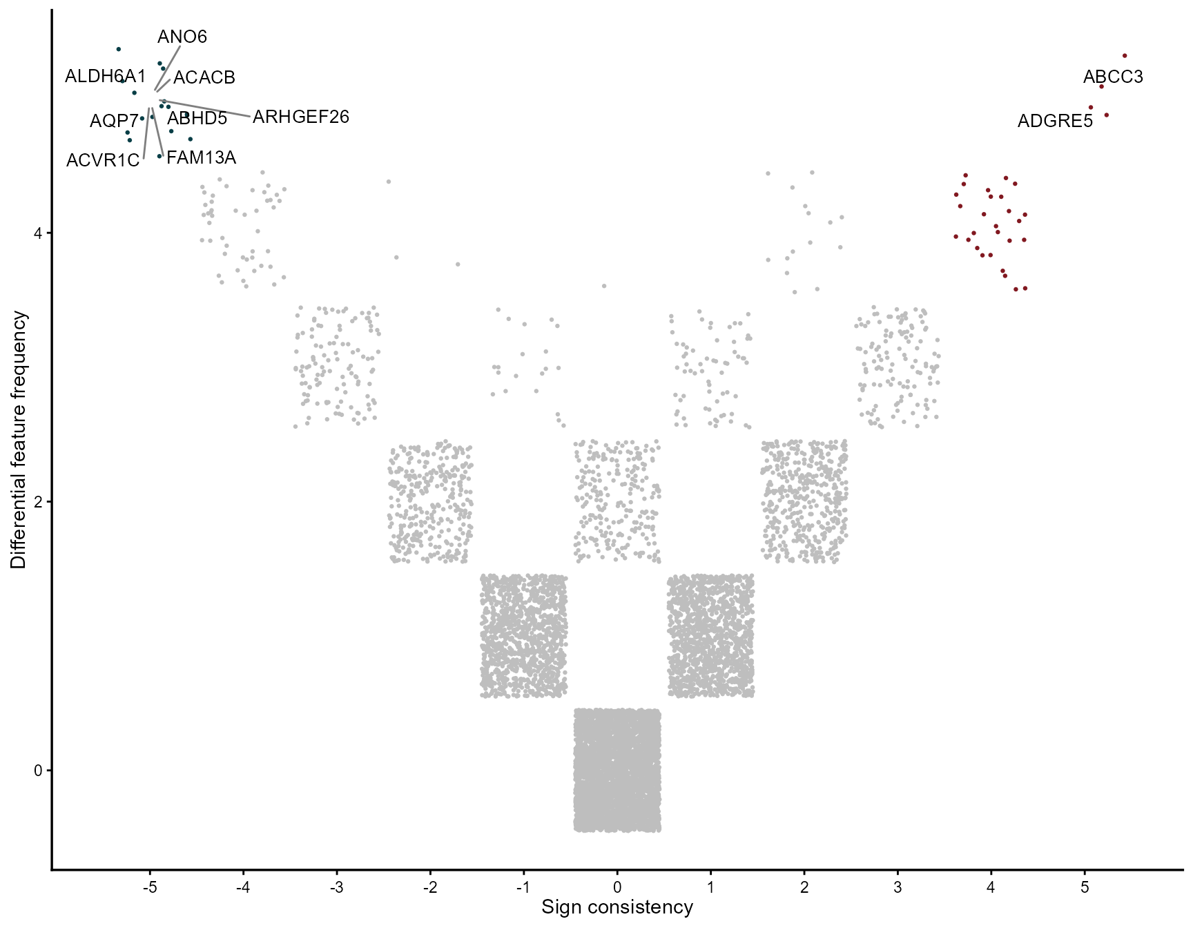

Feature barplot

draw_featurebar() accepts a colors parameter (see Customizing your plots) and, via mv_vote@featurefreq, also shows the inverse cumulative distribution of consistently perturbed features:

mv_vote@featurefreq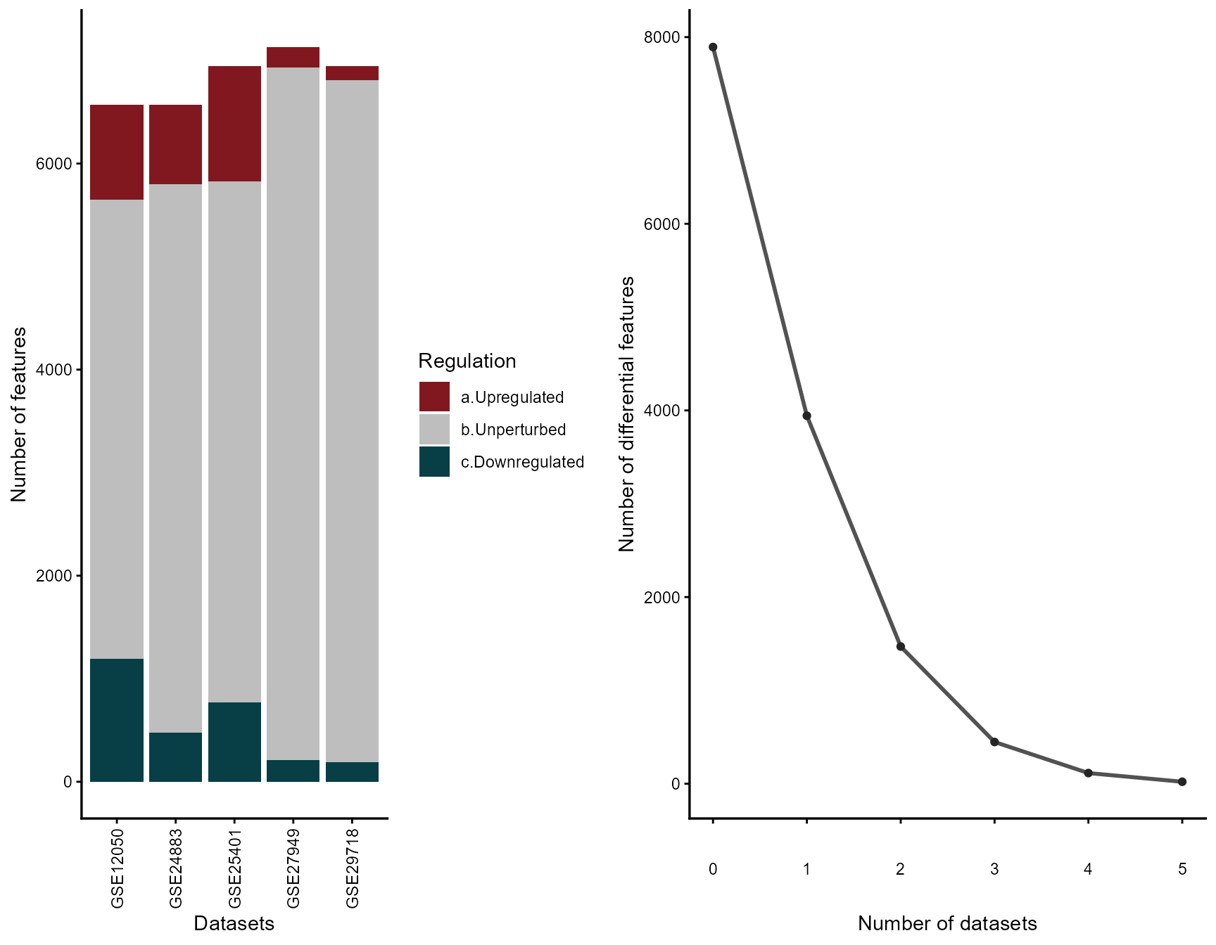

3. Combining approach (Fisher’s method)

The combining MetaVolcano summarizes a feature’s fold-change across studies by mean or median, and combines its per-study p-values with Fisher’s method. As with the REM, the result now also reports metap.adjust — metap corrected for multiple testing (default Benjamini-Hochberg, configurable via fdr_method) — which is what should drive feature selection rather than the nominal metap.

mv_fisher <- combining_mv(
  diffexp       = diffexplist,
  pcriteria     = "pvalue",
  foldchangecol = "Log2FC",
  genenamecol   = "Symbol",
  metafc        = "Mean",
  metathr       = 0.01,
  collaps       = TRUE,
  jobname       = "Fisher_example",
  outputfolder  = tempdir(),
  draw          = "HTML"
)

head(mv_fisher@metaresult, 3)

##   Symbol        metap metap.adjust     metafc       idx
## 1   MMP9 9.002947e-15 3.912045e-12  1.9693517  27.66076
## 2 ACVR1C 3.548802e-20 8.738332e-17 -1.2544105 -24.39818
## 3    ANG 5.674270e-26 4.191583e-22 -0.9364936 -23.64280

mv_fisher@MetaVolcano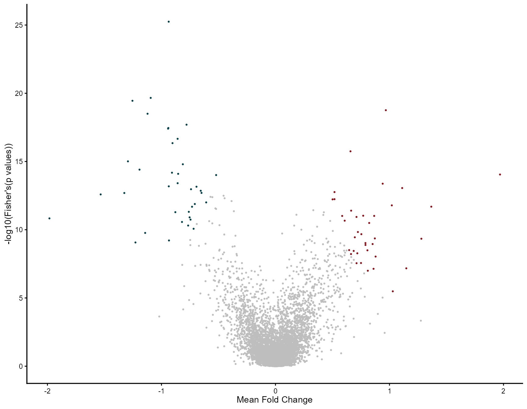

4. Functional enrichment — `enrichment_mv()`

enrichment_mv() wraps fGSEA and integrates directly with a REM MetaVolcano result. Gene sets can be supplied manually or downloaded automatically from MSigDB via msigdbr. It automatically ranks by the FDR-adjusted randomP.adjust when present (falling back to randomP with a message for REM results produced by an older package version).

# GO Biological Process (default category = "C5")
enrich <- enrichment_mv(mv_rem, subcategory = "GO:BP")
enrich$plot
head(enrich$result)

Three ranking strategies are available:

Ranking	Formula	Best for
`fc`	`randomSummary`	Pathways with large effects
`signed_p`	`-log10(p) × sign(FC)`	Pathways with consistent significance
`weighted_fc`	`FC × -log10(p)`	Balanced detection

enrich_fc  <- enrichment_mv(mv_rem, ranking = "fc")
enrich_sp  <- enrichment_mv(mv_rem, ranking = "signed_p")
enrich_wfc <- enrichment_mv(mv_rem, ranking = "weighted_fc")

enrich <- enrichment_mv(
  mv_rem,
  category            = "C5",
  subcategory         = "GO:BP",
  ranking             = "weighted_fc",
  plot_padj           = 0.05,
  plot_top_n          = 20,
  clean_pathway_names = TRUE,
  colors              = c(down = "navy", up = "darkred"),
  plot_title          = "GO:BP Enrichment (weighted FC ranking)"
)
enrich$plot

Custom gene sets are also supported directly:

my_pathways <- list(
  "INFLAMMATION" = c("IL6", "TNF", "IL1B", "CXCL8", "CCL2"),
  "ANGIOGENESIS" = c("VEGFA", "FLT1", "KDR", "ANGPT1"),
  "ECM_REMODEL"  = c("MMP2", "MMP9", "MMP12", "COL1A1")
)

enrich_custom <- enrichment_mv(mv_rem, pathways = my_pathways, clean_pathway_names = FALSE)

Additional example: differentially methylated probes

MetaVolcanoR is feature-agnostic: the same three strategies used above for genes apply directly to Illumina methylation microarray probes, or any other feature type described by an identifier, a log fold-change, a p-value, and a confidence interval. This section simulates four Illumina 450k datasets following the format of limma’s differential methylation output, to show the full workflow end to end.

library(IlluminaHumanMethylation450kanno.ilmn12.hg19)
library(tibble)
library(tidyr)
library(purrr)

For instructive purposes we use a subset of the 450k probe IDs (the first 1000) to generate simulated per-probe results across 4 datasets:

ann450k    <- getAnnotation(IlluminaHumanMethylation450kanno.ilmn12.hg19)
ann450k_df <- as.data.frame(ann450k) %>%
  rownames_to_column(var = "Probe_ID")

simulatedResults <- purrr::map_dfr(1:4, ~
  tibble::tibble(
    dataset = paste0("dataset_", .x),
    probes  = ann450k_df$Probe_ID[1:1000]
  ) %>%
  dplyr::mutate(
    logFC     = rnorm(dplyr::n(), mean = -0.01, sd = 1),
    AveExpr   = rnorm(dplyr::n(), mean = -0.75, sd = 2.5),
    t         = rnorm(dplyr::n(), mean = -0.2, sd = 2),
    P.Value   = runif(dplyr::n(), min = 0, max = 1),
    adj.P.Val = p.adjust(P.Value, method = "BH"),
    B         = rnorm(dplyr::n(), mean = -4.00, sd = 3.5),
    deltaBeta = rnorm(dplyr::n(), mean = -0.001, sd = 0.05)
  )
)

head(simulatedResults)

## # A tibble: 6 × 9
##   dataset   probes      logFC AveExpr      t P.Value adj.P.Val     B deltaBeta
##   <chr>     <chr>       <dbl>   <dbl>  <dbl>   <dbl>     <dbl> <dbl>     <dbl>
## 1 dataset_1 cg00050873 -1.83   -0.491 -0.836   0.434     0.976 -4.43   -0.121 
## 2 dataset_1 cg00212031 -0.257  -2.51   0.416   0.831     0.976 -4.85    0.0321
## 3 dataset_1 cg00213748 -0.254   2.99   1.40    0.246     0.976 -1.52    0.0130
## 4 dataset_1 cg00214611 -0.293  -1.51   3.30    0.410     0.976 -5.68   -0.0998
## 5 dataset_1 cg00455876 -0.564  -4.19   0.331   0.827     0.976 -5.11    0.0238
## 6 dataset_1 cg01707559  0.619   1.46   0.434   0.131     0.976 -2.21    0.0667

MetaVolcanoR needs a standard error and a fold-change confidence interval. Since limma’s moderated t-statistic is t = logFC / SE, we recover SE = logFC / t and approximate the 95% CI as logFC ± 1.96 * SE — exactly the same relationship used for prepare_swish() and prepare_geo2r() above. Results are then split by dataset into a named list, meta_input:

meta_input <- simulatedResults %>%
  dplyr::filter(!is.na(t) & t != 0) %>%
  dplyr::mutate(
    SE   = abs(logFC / t),
    CI.L = logFC - (1.96 * SE),
    CI.R = logFC + (1.96 * SE)
  ) %>%
  dplyr::select(probes, logFC, P.Value, CI.L, CI.R, dataset) %>%
  dplyr::group_split(dataset) %>%
  purrr::set_names(purrr::map_chr(., ~ unique(.x$dataset))) %>%
  purrr::map(as.data.frame)

str(meta_input, max.level = 1)

## List of 4
##  $ dataset_1:'data.frame':   1000 obs. of  6 variables:
##  $ dataset_2:'data.frame':   1000 obs. of  6 variables:
##  $ dataset_3:'data.frame':   1000 obs. of  6 variables:
##  $ dataset_4:'data.frame':   1000 obs. of  6 variables:

Once formatted, all three MetaVolcanoR strategies apply exactly as with gene-level data:

mv_rem_meth <- rem_mv(
  diffexp       = meta_input,
  pcriteria     = "P.Value",
  foldchangecol = "logFC",
  genenamecol   = "probes",
  llcol         = "CI.L",
  rlcol         = "CI.R",
  metathr       = 0.01,
  label_top_n   = 5,
  jobname       = "REM_methylation",
  outputfolder  = tempdir(),
  draw          = "HTML"
)

##   index     probes    logFC_1      CI.L_1     CI.R_1         vi_1    logFC_2
## 1   569 cg04765675  0.7815341 -26.9654056 28.5284739 200.40937763  0.9268912
## 2   316 cg02875834  1.0074911   0.4976544  1.5173277   0.06766280  1.4005463
## 3   327 cg02932805  1.3094563   0.7286222  1.8902904   0.08781973 -2.3525485
## 4   451 cg03962769 -0.7923792  -1.2610659 -0.3236925   0.05718118 -0.7637507
## 5     2 cg00011200 -1.0667369  -2.3568037  0.2233300   0.43322377  0.5516182
## 6   806 cg06443675 -0.8071532 -12.4660731 10.8517666  35.38380161 -0.8318084
##      CI.L_2     CI.R_2        vi_2    logFC_3    CI.L_3     CI.R_3       vi_3
## 1 -2.147915  4.0016975  2.46106679 -1.9837808 -2.609256 -1.3583059 0.10183749
## 2  0.662704  2.1383886  0.14171472  1.8967413  0.978854  2.8146286 0.21931412
## 3 -7.457415  2.7523177  6.78354305  0.8283869 -1.655747  3.3125210 1.60634173
## 4 -1.070311 -0.4571901  0.02446361 -1.1845005 -3.880508  1.5115068 1.89203859
## 5 -6.548362  7.6515983 13.12206308 -1.0007705 -1.386479 -0.6150615 0.03872642
## 6 -1.120699 -0.5429180  0.02172472 -0.7039417 -2.851169  1.4432853 1.20017270
##      logFC_4      CI.L_4     CI.R_4      vi_4 signcon ntimes randomSummary
## 1 -1.9217914 -3.09542395 -0.7481589 0.3585520       0      4    -1.8786052
## 2  0.8038212 -0.12520414  1.7328465 0.2246689       4      4     1.2117344
## 3  1.5960039  0.05532335  3.1366845 0.6178927       2      4     1.2821919
## 4 -0.7344246 -6.68179864  5.2129495 9.2074288      -4      4    -0.7759511
## 5  0.8742309 -1.94121201  3.6896738 2.0633899       0      4    -0.9702827
## 6 -0.5571805 -1.50026909  0.3859082 0.2315223      -4      4    -0.8065518
##   randomCi.lb randomCi.ub      randomP     het_QE   het_QEp   het_QM
## 1  -2.4217863  -1.3354242 1.213588e-11 3.34726359 0.3411184 45.94921
## 2   0.8296784   1.5937904 5.091762e-10 3.74360631 0.2905142 38.64177
## 3   0.7541098   1.8102739 1.947233e-06 2.24360250 0.5234112 22.64641
## 4  -1.0311114  -0.5207909 2.517479e-09 0.09920998 0.9919321 35.52539
## 5  -1.3361916  -0.6043737 2.022622e-07 1.87084197 0.5996416 27.01137
## 6  -1.0804351  -0.5326686 7.840685e-09 0.30673184 0.9587575 33.31423
##        het_QMp error randomP.adjust        se rank
## 1 1.213588e-11 FALSE   1.213588e-08 0.2771332    1
## 2 5.091762e-10 FALSE   1.697254e-07 0.1949265    2
## 3 1.947233e-06 FALSE   1.390881e-04 0.2694296    3
## 4 2.517479e-09 FALSE   6.293697e-07 0.1301838    4
## 5 2.022622e-07 FALSE   2.889461e-05 0.1866883    5
## 6 7.840685e-09 FALSE   1.568137e-06 0.1397364    6

mv_rem_meth@MetaVolcano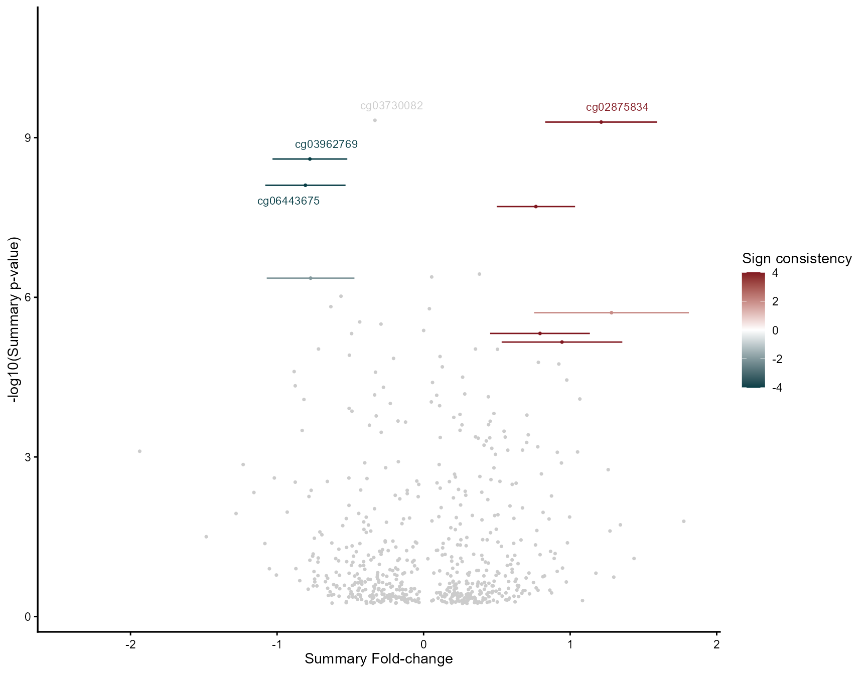

mv_vote_meth <- votecount_mv(
  diffexp       = meta_input,
  pcriteria     = "P.Value",
  foldchangecol = "logFC",
  genenamecol   = "probes",
  geneidcol     = NULL,
  pvalue        = 0.05,
  foldchange    = 0,
  metathr       = 0.01,
  label_top_n   = 10,
  label_size    = 3.5,
  jobname       = "Vote_methylation",
  outputfolder  = tempdir(),
  draw          = "HTML"
)

mv_vote_meth@MetaVolcano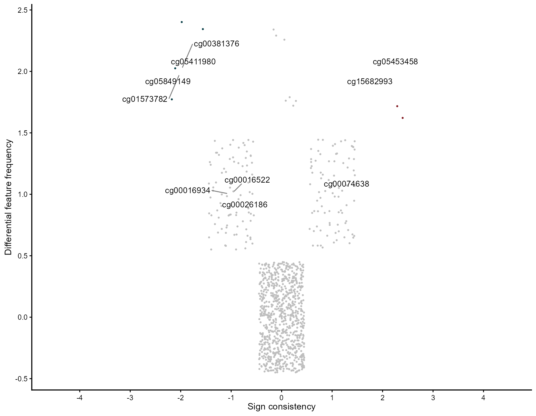

mv_fisher_meth <- combining_mv(
  diffexp       = meta_input,
  pcriteria     = "P.Value",
  foldchangecol = "logFC",
  genenamecol   = "probes",
  metafc        = "Mean",
  metathr       = 0.01,
  collaps       = TRUE,
  jobname       = "Fisher_methylation",
  outputfolder  = tempdir(),
  draw          = "HTML"
)

mv_fisher_meth@MetaVolcano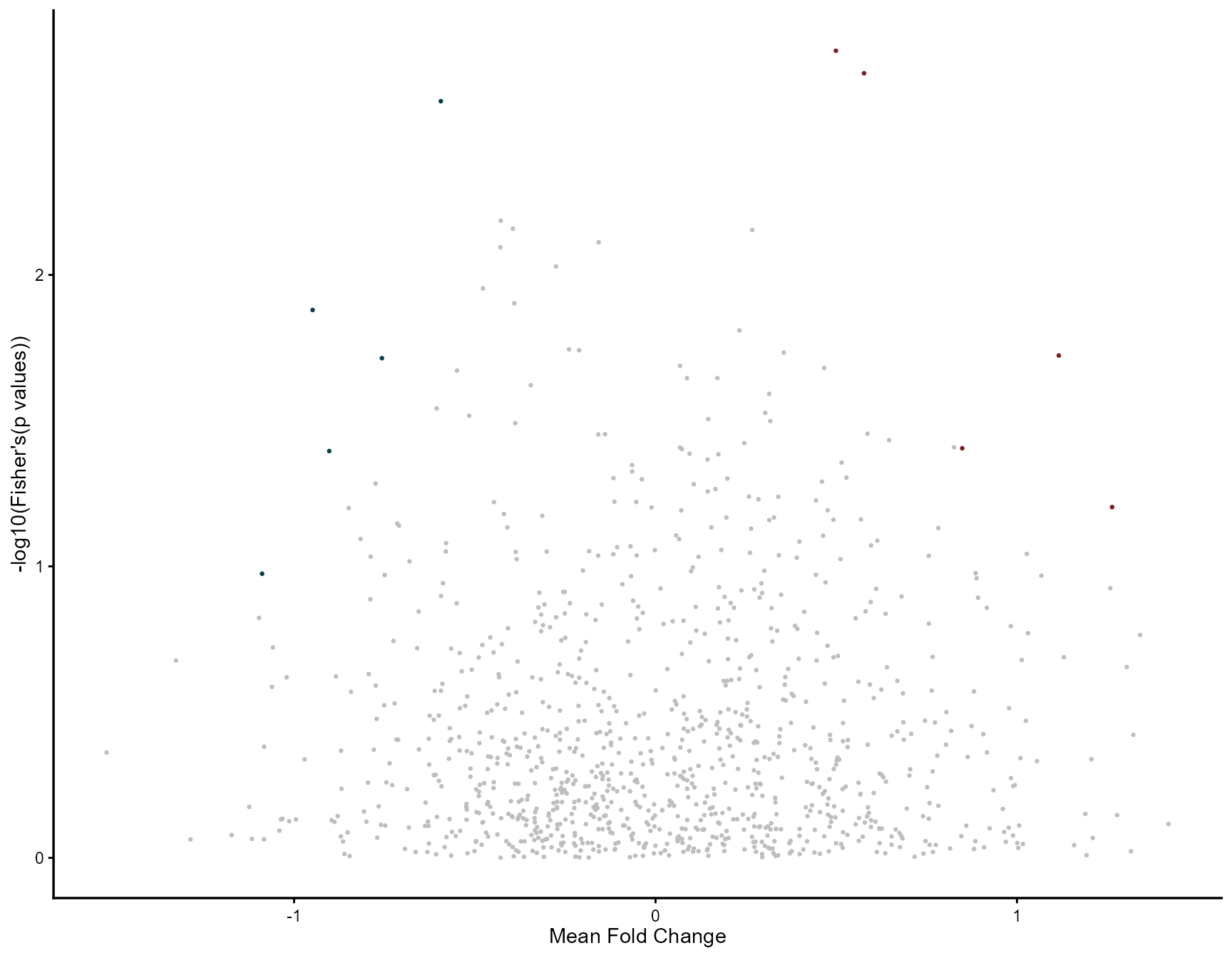

Since getAnnotation(IlluminaHumanMethylation450kanno.ilmn12.hg19) also retrieves probe metadata — which genomic feature each probe overlaps (promoter, gene body, TSS, UTRs) — it’s straightforward to filter for features of interest before running the meta-analysis, if a specific regulatory context is the target of the study.

Customizing your plots

Every example above uses MetaVolcanoR’s default styling — no custom colors, no titles, one consistent figure size. All three main functions (rem_mv(), votecount_mv(), combining_mv()), plus draw_forest() and draw_featurebar(), also accept a set of customization parameters, useful when preparing figures for a manuscript or a presentation.

Basic customization options

colors — custom color scheme
point_size — size of data points
label_genes — vector of specific features to label
label_top_n — automatically label the top N features
label_size — size of feature labels
plot_title — custom plot title (NULL for no title, the default)
show_legend — show or hide the legend

Example 1: custom colors and feature labels

meta_custom <- rem_mv(
  diffexp       = diffexplist,
  metathr       = 0.01,
  outputfolder  = tempdir(),
  draw          = "HTML",
  colors        = c(low = "purple", mid = "white", high = "orange", na = "gray80"),
  point_size    = 1.5,
  label_genes   = c("MMP9", "COL6A6", "MXRA5", "CIDEA"),
  label_size    = 4,
  plot_title    = "REM Meta-Analysis - Custom Colors",
  show_legend   = TRUE
)

##   index  Symbol   Log2FC_1     CI.L_1     CI.R_1       vi_1   Log2FC_2
## 1  4795   MXRA5  0.8150851  0.3109324  1.3192377 0.06616251  1.3001104
## 2  2166  COL6A6 -1.7480348 -2.5780749 -0.9179947 0.17934364 -0.8388366
## 3  2053   CIDEA         NA         NA         NA         NA         NA
## 4  7115 SULT1A4  0.9689025  0.5103475  1.4274575 0.05473571  0.7513323
## 5   130   ACACB -0.8431142 -1.4708480 -0.2153804 0.10257437 -1.1119841
## 6  6528 SLC27A2 -0.6782948 -0.9931027 -0.3634869 0.02579759 -1.8916655
##       CI.L_2     CI.R_2       vi_2   Log2FC_3     CI.L_3     CI.R_3        vi_3
## 1  0.6603306  1.9398901 0.10654886  1.1895480  0.8401301  1.5389659 0.031781777
## 2 -1.3578456 -0.3198277 0.07011930 -1.0300519 -1.4730328 -0.5870710 0.051080819
## 3         NA         NA         NA -1.0111528 -1.3226326 -0.6996729 0.025255027
## 4  0.4707021  1.0319624 0.02050012         NA         NA         NA          NA
## 5 -1.7417389 -0.4822293 0.10323592 -0.5305046 -0.6957455 -0.3652637 0.007107599
## 6 -2.6822584 -1.1010726 0.16270229 -1.2126830 -1.6702908 -0.7550753 0.054509799
##     Log2FC_4    CI.L_4     CI.R_4      vi_4   Log2FC_5     CI.L_5     CI.R_5
## 1  0.2188594 -1.052230  1.4899492 0.4205720  0.8051543  0.1367255  1.4735830
## 2 -1.3755263 -2.162453 -0.5885999 0.1611967 -0.7213490 -1.5714484  0.1287505
## 3 -1.7991026 -2.918939 -0.6792665 0.3264351 -0.8738120 -1.6373061 -0.1103179
## 4         NA        NA         NA        NA         NA         NA         NA
## 5 -0.7991042 -1.457868 -0.1403403 0.1129659 -0.5155929 -0.8606782 -0.1705076
## 6 -1.3554403 -2.288444 -0.4224370 0.2265970 -1.4905464 -2.5565023 -0.4245905
##         vi_5 signcon ntimes randomSummary randomCi.lb randomCi.ub      randomP
## 1 0.11630493       5      5     1.0333001   0.7882044   1.2783958 1.420312e-16
## 2 0.18811668      -5      5    -1.0649749  -1.3396138  -0.7903361 2.956522e-14
## 3 0.15173972      -3      3    -1.0417876  -1.3210774  -0.7624977 2.653168e-13
## 4         NA       2      2     0.8106154   0.5712566   1.0499741 3.187477e-11
## 5 0.03099851      -5      5    -0.5830624  -0.7212245  -0.4449003 1.324963e-16
## 6 0.29577833      -5      5    -1.2207058  -1.6760435  -0.7653680 1.484852e-07
##      het_QE    het_QEp   het_QM      het_QMp error randomP.adjust         se
## 1  4.179945 0.38220032 68.27752 1.420312e-16 FALSE   3.737313e-13 0.12504883
## 2  4.580708 0.33308457 57.76318 2.956522e-14 FALSE   4.667756e-11 0.14012185
## 3  1.980047 0.37156797 53.44957 2.653168e-13 FALSE   3.490685e-10 0.14249482
## 4  0.629179 0.42765661 44.05825 3.187477e-11 FALSE   2.287450e-08 0.12212181
## 5  4.317851 0.36469506 68.41455 1.324963e-16 FALSE   3.737313e-13 0.07049086
## 6 11.099093 0.02547263 27.60901 1.484852e-07 FALSE   3.255949e-05 0.23231516
##   rank
## 1    1
## 2    2
## 3    3
## 4    4
## 5    5
## 6    6

meta_custom@MetaVolcano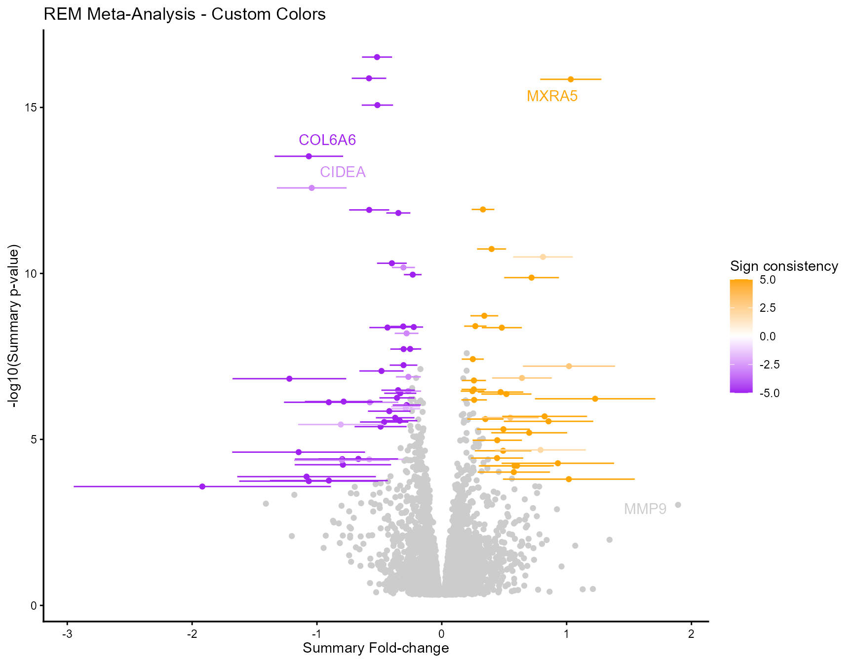

Example 2: highlighting top features automatically

meta_vote_labeled <- votecount_mv(
  diffexp       = diffexplist,
  pvalue        = 0.05,
  metathr       = 0.01,
  outputfolder  = tempdir(),
  draw          = "HTML",
  colors        = c("orange", "gray90", "purple"),
  point_size    = 1.2,
  label_top_n   = 10,
  label_size    = 3.5,
  plot_title    = "Vote-Counting: Top 10 Features Labeled"
)

meta_vote_labeled@MetaVolcano

Example 3: publication-ready figures

meta_publication <- combining_mv(
  diffexp       = diffexplist,
  metafc        = "Median",
  metathr       = 0.01,
  collaps       = TRUE,
  outputfolder  = tempdir(),
  draw          = "HTML",
  colors        = c("darkgreen", "white", "darkorange"),
  point_size    = 1.0,
  label_genes   = c("MMP9", "ANG", "ACVR1C"),
  label_size    = 3,
  plot_title    = NULL,   # No title, for publication
  show_legend   = FALSE
)

meta_publication@MetaVolcano

Example 4: customizing forest plots

draw_forest(
  remres        = mv_rem,
  gene          = "MMP9",
  outputfolder  = tempdir(),
  draw          = "PDF",
  colors        = c(
    positive  = "darkred",   # Positive fold-change
    negative  = "steelblue", # Negative fold-change
    neutral   = "gray70",    # Individual studies
    reference = "black"      # Reference line
  ),
  point_size    = 3,
  plot_width    = 7,   # inches, for PDF
  plot_height   = 6,
  plot_title    = "MMP9 Expression Meta-Analysis"
)

Color scheme examples

# Professional/conservative
colors_professional <- c(low = "blue", mid = "white", high = "red", na = "gray80")

# High contrast (for presentations)
colors_presentation <- c(low = "purple", mid = "white", high = "orange", na = "lightgray")

# Color-blind friendly
colors_colorblind <- c(low = "#0072B2", mid = "white", high = "#D55E00", na = "gray80")

# Grayscale (for print)
colors_grayscale <- c(low = "black", mid = "gray90", high = "gray30", na = "gray70")

meta_rem <- rem_mv(
  diffexp = diffexplist,
  colors  = colors_colorblind,  # or any of the schemes above
  # ... other parameters
)

For vote-counting and combining, provide a 3-color vector instead (down, neutral, up):

custom_colors <- c("navyblue", "gray85", "darkred")

meta_vote <- votecount_mv(
  diffexp = diffexplist,
  colors  = custom_colors,
  # ... other parameters
)

Combining multiple customizations

meta_final <- rem_mv(
  diffexp       = diffexplist,
  metathr       = 0.01,
  outputfolder  = tempdir(),
  draw          = "HTML",
  ncores        = 4,
  colors        = c(low = "#0072B2", mid = "white", high = "#D55E00", na = "gray80"),
  point_size    = 1.5,
  label_genes   = c("MMP9", "COL6A6"),
  label_top_n   = 5,
  label_size    = 3.5,
  plot_title    = "Meta-Analysis: Disease vs Control",
  show_legend   = TRUE
)

meta_final@MetaVolcano

draw_forest(
  remres        = meta_final,
  gene          = "MMP9",
  outputfolder  = tempdir(),
  draw          = "PDF",
  colors        = c(positive = "#D55E00", negative = "#0072B2",
                    neutral = "gray60", reference = "black"),
  point_size    = 3,
  plot_width    = 8,
  plot_height   = 6
)

Tips for publication-quality figures

Use color-blind friendly palettes (see examples above).
Set show_legend = FALSE for cleaner figures (add a legend in the figure caption instead).
Label only key features rather than showing every label.
Use plot_title = NULL and add titles in your manuscript text instead.
Save as PDF (draw = "PDF") for vector graphics in publications.
Adjust plot_width and plot_height to match journal requirements.
Use consistent colors across all figures in a given paper.

Saving plots separately

meta_result <- rem_mv(
  diffexp      = diffexplist,
  draw         = "HTML",  # or "PDF"
  outputfolder = "path/to/output"
  # ... other parameters
)

# The plot is automatically saved to outputfolder.
# HTML: interactive plot you can explore in a browser.
# PDF: publication-ready vector graphics.

sessionInfo()

## R version 4.4.1 (2024-06-14 ucrt)
## Platform: x86_64-w64-mingw32/x64
## Running under: Windows 11 x64 (build 26200)
## 
## Matrix products: default
## 
## 
## locale:
## [1] LC_COLLATE=Portuguese_Brazil.utf8  LC_CTYPE=Portuguese_Brazil.utf8   
## [3] LC_MONETARY=Portuguese_Brazil.utf8 LC_NUMERIC=C                      
## [5] LC_TIME=Portuguese_Brazil.utf8    
## 
## time zone: America/Sao_Paulo
## tzcode source: internal
## 
## attached base packages:
## [1] parallel  stats4    stats     graphics  grDevices utils     datasets 
## [8] methods   base     
## 
## other attached packages:
##  [1] purrr_1.2.2                                       
##  [2] tidyr_1.3.2                                       
##  [3] tibble_3.3.1                                      
##  [4] IlluminaHumanMethylation450kanno.ilmn12.hg19_0.6.1
##  [5] minfi_1.52.1                                      
##  [6] bumphunter_1.48.0                                 
##  [7] locfit_1.5-9.12                                   
##  [8] iterators_1.0.14                                  
##  [9] foreach_1.5.2                                     
## [10] Biostrings_2.74.1                                 
## [11] XVector_0.46.0                                    
## [12] SummarizedExperiment_1.36.0                       
## [13] Biobase_2.66.0                                    
## [14] MatrixGenerics_1.18.1                             
## [15] matrixStats_1.5.0                                 
## [16] GenomicRanges_1.58.0                              
## [17] GenomeInfoDb_1.42.3                               
## [18] IRanges_2.40.1                                    
## [19] S4Vectors_0.44.0                                  
## [20] BiocGenerics_0.52.0                               
## [21] ggplot2_4.0.3                                     
## [22] dplyr_1.2.1                                       
## [23] MetaVolcanoR_1.0.2                                
## 
## loaded via a namespace (and not attached):
##   [1] splines_4.4.1             BiocIO_1.16.0            
##   [3] bitops_1.0-9              preprocessCore_1.68.0    
##   [5] XML_3.99-0.23             lifecycle_1.0.5          
##   [7] Rdpack_2.6.6              lattice_0.22-6           
##   [9] MASS_7.3-60.2             base64_2.0.2             
##  [11] scrime_1.3.7              crosstalk_1.2.2          
##  [13] magrittr_2.0.4            limma_3.62.2             
##  [15] metafor_5.0-1             plotly_4.12.0            
##  [17] sass_0.4.10               rmarkdown_2.31           
##  [19] plotrix_3.8-14            jquerylib_0.1.4          
##  [21] yaml_2.3.12               qqconf_1.3.2             
##  [23] otel_0.2.0                sn_2.1.3                 
##  [25] doRNG_1.8.6.3             askpass_1.2.1            
##  [27] cowplot_1.2.0             DBI_1.3.0                
##  [29] RColorBrewer_1.1-3        multcomp_1.4-30          
##  [31] abind_1.4-8               zlibbioc_1.52.0          
##  [33] quadprog_1.5-8            RCurl_1.98-1.18          
##  [35] TH.data_1.1-5             sandwich_3.1-1           
##  [37] GenomeInfoDbData_1.2.13   ggrepel_0.9.8            
##  [39] rentrez_1.2.4             genefilter_1.88.0        
##  [41] TFisher_0.2.0             annotate_1.84.0          
##  [43] pkgdown_2.2.0             DelayedMatrixStats_1.28.1
##  [45] codetools_0.2-20          DelayedArray_0.32.0      
##  [47] xml2_1.5.2                tidyselect_1.2.1         
##  [49] UCSC.utils_1.2.0          farver_2.1.2             
##  [51] beanplot_1.3.1            illuminaio_0.48.0        
##  [53] mathjaxr_2.0-0            GenomicAlignments_1.42.0 
##  [55] jsonlite_2.0.0            multtest_2.62.0          
##  [57] survival_3.6-4            systemfonts_1.3.2        
##  [59] tools_4.4.1               ragg_1.5.2               
##  [61] Rcpp_1.1.1                glue_1.8.0               
##  [63] mnormt_2.1.2              SparseArray_1.6.2        
##  [65] xfun_0.57                 metap_1.14               
##  [67] HDF5Array_1.34.0          withr_3.0.3              
##  [69] numDeriv_2016.8-1.1       fastmap_1.2.0            
##  [71] rhdf5filters_1.18.1       openssl_2.4.0            
##  [73] digest_0.6.35             R6_2.6.1                 
##  [75] textshaping_1.0.5         colorspace_2.1-2         
##  [77] RSQLite_2.4.6             utf8_1.2.6               
##  [79] generics_0.1.4            data.table_1.18.2.1      
##  [81] rtracklayer_1.66.0        httr_1.4.8               
##  [83] htmlwidgets_1.6.4         S4Arrays_1.6.0           
##  [85] pkgconfig_2.0.3           gtable_0.3.6             
##  [87] blob_1.3.0                S7_0.2.1                 
##  [89] siggenes_1.80.0           htmltools_0.5.8.1        
##  [91] scales_1.4.0              png_0.1-9                
##  [93] knitr_1.51                tzdb_0.5.0               
##  [95] rjson_0.2.23              nlme_3.1-164             
##  [97] curl_7.0.0                zoo_1.8-15               
##  [99] cachem_1.1.0              rhdf5_2.50.2             
## [101] metadat_1.6-0             AnnotationDbi_1.68.0     
## [103] restfulr_0.0.16           desc_1.4.3               
## [105] GEOquery_2.74.0           pillar_1.11.1            
## [107] grid_4.4.1                reshape_0.8.10           
## [109] vctrs_0.7.1               xtable_1.8-8             
## [111] evaluate_1.0.5            readr_2.2.0              
## [113] GenomicFeatures_1.58.0    mvtnorm_1.3-5            
## [115] cli_3.6.2                 compiler_4.4.1           
## [117] Rsamtools_2.22.0          rlang_1.2.0              
## [119] crayon_1.5.3              rngtools_1.5.2           
## [121] mutoss_0.1-14             labeling_0.4.3           
## [123] nor1mix_1.3-3             mclust_6.1.3             
## [125] plyr_1.8.9                fs_2.1.0                 
## [127] viridisLite_0.4.3         BiocParallel_1.40.0      
## [129] assertthat_0.2.1          topconfects_1.22.0       
## [131] lazyeval_0.2.3            Matrix_1.7-0             
## [133] hms_1.1.4                 sparseMatrixStats_1.18.0 
## [135] bit64_4.6.0-1             Rhdf5lib_1.28.0          
## [137] KEGGREST_1.46.0           statmod_1.5.1            
## [139] rbibutils_2.4.1           memoise_2.0.1            
## [141] bslib_0.11.0              bit_4.6.0

Izabela Mamede, Bárbara Marinho, Cesar Prada, Carlos Mata-Machado, Helder Nakaya

2026-07-20

Introduction: Why Meta-Analysis?

Overview

Load library

Preparing Your Data

What do you have?

CI ready

Standard error (SE)

Variance directly

Test statistic (z or t)

DESeq2

limma

edgeR

Swish/fishpond (transcript-level)

GEO2R

Checking your data is correctly formatted

Implemented meta-analysis approaches

1. Random Effects Model (REM)

Labeling top features

Forest plots

2. Vote-counting approach

Feature barplot

3. Combining approach (Fisher’s method)

4. Functional enrichment — `enrichment_mv()`

Additional example: differentially methylated probes

Customizing your plots

Basic customization options

Example 1: custom colors and feature labels

Example 2: highlighting top features automatically

Example 3: publication-ready figures

Example 4: customizing forest plots

Color scheme examples

Combining multiple customizations

Tips for publication-quality figures

Saving plots separately

MetaVolcanoR: gene and transcript-level meta-analysis

Izabela Mamede, Bárbara Marinho, Cesar Prada, Carlos Mata-Machado, Helder Nakaya

2026-07-20

Introduction: Why Meta-Analysis?

Overview

Load library

Preparing Your Data

What do you have?

CI ready

Standard error (SE)

Variance directly

Test statistic (z or t)

DESeq2

limma

edgeR

Swish/fishpond (transcript-level)

GEO2R

Checking your data is correctly formatted

Implemented meta-analysis approaches

1. Random Effects Model (REM)

Labeling top features

Forest plots

2. Vote-counting approach

Feature barplot

3. Combining approach (Fisher’s method)

4. Functional enrichment — enrichment_mv()

Additional example: differentially methylated probes

Customizing your plots

Basic customization options

Example 1: custom colors and feature labels

Example 2: highlighting top features automatically

Example 3: publication-ready figures

Example 4: customizing forest plots

Color scheme examples

Combining multiple customizations

Tips for publication-quality figures

Saving plots separately

4. Functional enrichment — `enrichment_mv()`